Code Snippets

The following code snippets demonstrate how to use the basic objects and methods of SigAlg. This page is not yet comprehensive, so the user will need to inspect the API reference for additional code examples. More code snippets will be added to this page as they are written.

It is also worth checking out the extended introduction to SigAlg.

Sample spaces

Creating sample spaces

API References: SampleSpace

create_sample_space.pyOutput

"""Instantiate a SampleSpace from different data sources."""

import pandas as pd

from sigalg.core import SampleSpace

Omega_from_list = SampleSpace(  # (1)!
    name="Omega_from_list",
).from_list(["H", "T"])

Omega_from_sequence = SampleSpace(  # (2)!
    name="Omega_from_sequence",
).from_sequence(size=6, initial_index=1)

Omega_with_prefixes = SampleSpace(  # (3)!
    name="Omega_with_prefixes",
).from_sequence(size=4, prefix="omega")

data = pd.Index(["red", "green", "blue"])
Omega_from_pandas = SampleSpace(  # (4)!
    name="Omega_from_pandas",
).from_pandas(data)

print(Omega_from_list)
print("\n", Omega_from_sequence)
print("\n", Omega_with_prefixes)
print("\n", Omega_from_pandas)

1. Create a sample space \(\Omega = \{H, T\}\) from a Python list.
2. Create a sample space \(\Omega = \{1, 2, 3, 4, 5, 6\}\) using the from_sequence method.
3. Create a sample space \(\Omega = \{\omega_0, \omega_1, \omega_2, \omega_3\}\) using the from_sequence method with a prefix.
4. Create a sample space \(\Omega = \{\text{red}, \text{green}, \text{blue}\}\) from a pd.Index with the from_pandas method.

Sample space 'Omega_from_list':
['H', 'T']

 Sample space 'Omega_from_sequence':
[1, 2, 3, 4, 5, 6]

 Sample space 'Omega_with_prefixes':
['omega_0', 'omega_1', 'omega_2', 'omega_3']

 Sample space 'Omega_from_pandas':
['red', 'green', 'blue']

Extracting events

API References: SampleSpace

extract_event.pyOutput

"""Extracting events from a sample space."""

from sigalg.core import SampleSpace

Omega = SampleSpace().from_sequence(size=5, initial_index=1, prefix="omega")  # (1)!

A = Omega.get_event(["omega_1", "omega_2", "omega_3"], name="A")  # (2)!
B = Omega[2:5, "B"]  # (3)!
C = Omega[[0, 3], "C"]  # (4)!

print(Omega)
print("\n", A)
print("\n", B)
print("\n", C)

1. Create a sample space \(\Omega = \{\omega_1, \omega_2, \omega_3, \omega_4, \omega_5\}\).
2. Extract the event \(A=\{\omega_1, \omega_2, \omega_3\}\) using the get_event method.
3. Extract the event \(B=\{\omega_3, \omega_4, \omega_5\}\) by (positional-based) slicing.
4. Extract the event \(C=\{\omega_1, \omega_4\}\) by (positional-based) indexing.

Sample space 'Omega':
['omega_1', 'omega_2', 'omega_3', 'omega_4', 'omega_5']

 Event 'A':
['omega_1', 'omega_2', 'omega_3']

 Event 'B':
['omega_3', 'omega_4', 'omega_5']

 Event 'C':
['omega_1', 'omega_4']

Creating probability spaces

API References: ProbabilityMeasure, SampleSpace, SigmaAlgebra

create_prob_space.pyOutput

"""Create a ProbabilitySpace from an instance of SampleSpace, SigmaAlgebra, and ProbabilityMeasure."""

from sigalg.core import ProbabilityMeasure, SampleSpace, SigmaAlgebra

Omega = SampleSpace().from_sequence(size=4)  # (1)!

atom_ids = {
    0: 0,
    1: 1,
    2: 0,
    3: 1,
}
F = SigmaAlgebra(sample_space=Omega).from_dict(atom_ids)  # (2)!

probabilities = {
    0: 0.1,
    1: 0.2,
    2: 0.4,
    3: 0.3,
}
P = ProbabilityMeasure(sample_space=Omega).from_dict(probabilities)  # (3)!

prob_space = Omega.make_probability_space(  # (4)!
    sigma_algebra=F,
    probability_measure=P,
)

print(prob_space)

1. Create a sample space \(\Omega = \{0,1,2,3\}\).
2. Create a \(\sigma\)-algebra \(\mathcal{F}\) on \(\Omega\) with atoms \(A_0 = \{0,2\}\) and \(A_1 = \{1,3\}\).
3. Create a probability measure \(P\) on \(\Omega\) with \(P(\{\omega\}) = \begin{cases} 0.1 & \text{if } \omega = 0 \\ 0.2 & \text{if } \omega = 1 \\ 0.4 & \text{if } \omega = 2 \\ 0.3 & \text{if } \omega = 3 \end{cases}\)
4. Create a probability space \((\Omega, \mathcal{F}, P)\).

Probability space (Omega, F, P)
===============================

* Sample space 'Omega':
[0, 1, 2, 3]

* Sigma algebra 'F':
        atom ID
sample         
0             0
1             1
2             0
3             1

* Probability measure 'P':
        probability
sample             
0               0.1
1               0.2
2               0.4
3               0.3

Accessing underlying data

API References: SampleSpace

sample_space_data.pyOutput

"""Accessing the underlying data in a sample space."""

from sigalg.core import SampleSpace

Omega = SampleSpace().from_sequence(size=5, prefix="s")  # (1)!

data = Omega.data  # (2)!

print(Omega)
print("\nThe `data` attribute of the sample space:\n", Omega.data)

1. Create a sample space \(\Omega = \{s_0,s_1,s_2,s_3,s_4\}\).
2. Access the underlying data of the sample space as a pd.Index using the data attribute.

Sample space 'Omega':
['s_0', 's_1', 's_2', 's_3', 's_4']

The `data` attribute of the sample space:
 Index(['s_0', 's_1', 's_2', 's_3', 's_4'], dtype='str', name='sample')

Events

Set operations

API References: Event, SampleSpace

set_operations.pyOutput

"""Perform set-theoretic operations on events."""

from sigalg.core import SampleSpace

Omega = SampleSpace().from_sequence(size=5)  # (1)!

A = Omega.get_event([0, 1, 2], name="A")
B = Omega.get_event([2, 3, 4], name="B")

intersection = A & B
union = A | B
difference = A - B
complement = ~A

print(A)
print("\n", B)
print("\n", intersection)
print("\n", union)
print("\n", difference)
print("\n", complement)

1. Create a sample space \(\Omega = \{0,1,2,3,4\}\).

Event 'A':
[0, 1, 2]

 Event 'B':
[2, 3, 4]

 Event 'A intersect B':
[2]

 Event 'A union B':
[0, 1, 2, 3, 4]

 Event 'A difference B':
[0, 1]

 Event 'A complement':
[3, 4]

Order operations

API References: Event, SampleSpace

order_operations.pyOutput

"""Perform order-theoretic operations on events."""

from sigalg.core import SampleSpace

Omega = SampleSpace().from_sequence(size=5)  # (1)!

A = Omega.get_event([0, 1, 2], name="A")
B = Omega.get_event([0, 1, 2, 3], name="B")
C = Omega.get_event([0, 1, 3], name="C")

print(A)
print("\n", B)
print("\n", C)
print("\nIs A a subset of B?", A <= B)
print("Is A a subset of C?", A <= C)
print("Is B a superset of A?", B >= A)
print("Is C a superset of A?", C >= A)

1. Create a sample space \(\Omega = \{0,1,2,3,4\}\).

Event 'A':
[0, 1, 2]

 Event 'B':
[0, 1, 2, 3]

 Event 'C':
[0, 1, 3]

Is A a subset of B? True
Is A a subset of C? False
Is B a superset of A? True
Is C a superset of A? False

Event spaces

Creating event spaces

API References: EventSpace, SampleSpace, SigmaAlgebra

create_event_space.pyOutput

"""Create an event space from a sample space and a sigma-algebra."""

from sigalg.core import EventSpace, SampleSpace, SigmaAlgebra

Omega = SampleSpace().from_sequence(size=4)  # (1)!

atom_ids = {
    0: 0,
    1: 0,
    2: 1,
    3: 2,
}
F = SigmaAlgebra(sample_space=Omega).from_dict(atom_ids)  # (2)!

event_space = EventSpace(sample_space=Omega, sigma_algebra=F)  # (3)!

print(event_space.sample_space)
print("\n", event_space.sigma_algebra)  # (4)!

new_atom_ids = {
    0: 0,
    1: 1,
    2: 1,
    3: 0,
}
G = SigmaAlgebra(sample_space=Omega, name="G").from_dict(new_atom_ids)  # (5)!

event_space.sigma_algebra = G  # (6)!

print("\n", event_space.sigma_algebra)

1. Create a sample space \(\Omega = \{0,1,2,3\}\).
2. Create a \(\sigma\)-algebra \(\mathcal{F}\) on \(\Omega\) with atoms \(A_0 = \{0,1\}\), \(A_1 = \{2\}, A_2 = \{3\}\).
3. Create an event space \((\Omega, \mathcal{F})\).
4. The sample space \(\Omega\) and \(\sigma\)-algebra \(\mathcal{F}\) are accessible as attributes of the event space.
5. Define a new \(\sigma\)-algebra \(\mathcal{G}\).
6. The sigma_algebra attribute of the event space is settable, so we can replace \(\mathcal{F}\) with \(\mathcal{G}\).

Sample space 'Omega':
[0, 1, 2, 3]

 Sigma algebra 'F':
        atom ID
sample         
0             0
1             0
2             1
3             2

 Sigma algebra 'G':
        atom ID
sample         
0             0
1             1
2             1
3             0

Event space inherited methods

API References: EventSpace, SampleSpace, SigmaAlgebra

event_space_methods.pyOutput

"""Event spaces inherit methods from SampleSpace and SigmaAlgebra."""

from sigalg.core import EventSpace, SampleSpace, SigmaAlgebra

Omega = SampleSpace().from_sequence(size=4)  # (1)!

atom_ids = {
    0: 0,
    1: 0,
    2: 1,
    3: 2,
}
F = SigmaAlgebra(sample_space=Omega).from_dict(atom_ids)  # (2)!

event_space = EventSpace(sample_space=Omega, sigma_algebra=F)  # (3)!

A = event_space.get_event([0, 3])  # (4)!
B = event_space.get_event([0, 1, 2])

print("Is the event A measurable?", event_space.is_measurable(A))  # (5)!
print("\nIs the event B measurable?", event_space.is_measurable(B))

1. Create a sample space \(\Omega = \{0,1,2,3\}\).
2. Create a \(\sigma\)-algebra \(\mathcal{F}\) on \(\Omega\) with atoms \(A_0 = \{0,1\}\), \(A_1 = \{2\}, A_2 = \{3\}\).
3. Create an event space \((\Omega, \mathcal{F})\)
4. The EventSpace inherits the method get_event from SampleSpace.
5. The EventSpace inherits the method is_measurable from SigmaAlgebra. The event \(A\) is not measurable, since it is not a union of atoms, but the event \(B\) is measurable, since it is a union of atoms.

Is the event A measurable? False

Is the event B measurable? True

\(\sigma\)-algebras

Creating \(\sigma\)-algebras

API References: SampleSpace, SigmaAlgebra

create_sigma_algebra.pyOutput

"""Create a sigma-algebra from a dictionary of atom IDs."""

from sigalg.core import SampleSpace, SigmaAlgebra

Omega = SampleSpace().from_sequence(size=5)  # (1)!

sample_id_to_atom_id = {  # (2)!
    0: 0,
    1: 1,
    2: 0,
    3: 1,
    4: 2,
}

F = SigmaAlgebra(sample_space=Omega).from_dict(sample_id_to_atom_id)  # (3)!

print(F)  # (4)!

1. Create a sample space \(\Omega = \{0,1,2,3,4\}\).
2. A \(\sigma\)-algebra \(\mathcal{F}\) on \(\Omega = \{0,1,2,3,4\}\) is determined by its minimal (with respect to subset inclusion) non-empty sets, called atoms. We will define \(\mathcal{F}\) by declaring its atoms to be \(A_0 = \{0,2\}\), \(A_1 = \{1,3\}\) and \(A_2 = \{4\}\). The dictionary on this line maps each sample point in \(\Omega\) to the the index of its atom.
3. Instantiate the \(\sigma\)-algebra \(\mathcal{F}\) with the dictionary.
4. Print the \(\sigma\)-algebra.

Sigma algebra 'F':
        atom ID
sample         
0             0
1             1
2             0
3             1
4             2

Probability spaces

Creating probability spaces

API References: ProbabilityMeasure, ProbabilitySpace, SampleSpace, SigmaAlgebra

create_probability_space.pyOutput

"""Create a probability space from a sample space, a sigma-algebra, and a probability measure."""

from sigalg.core import ProbabilityMeasure, ProbabilitySpace, SampleSpace, SigmaAlgebra

Omega = SampleSpace().from_sequence(size=4)  # (1)!

atom_ids = {
    0: 0,
    1: 0,
    2: 1,
    3: 2,
}
F = SigmaAlgebra(sample_space=Omega).from_dict(atom_ids)  # (2)!

probabilities = {
    0: 0.1,
    1: 0.2,
    2: 0.4,
    3: 0.3,
}
P = ProbabilityMeasure(sample_space=Omega).from_dict(probabilities)  # (3)!

prob_space = ProbabilitySpace(  # (4)!
    sample_space=Omega,
    sigma_algebra=F,
    probability_measure=P,
)

print(prob_space.sample_space)  # (5)!
print("\n", prob_space.sigma_algebra)
print("\n", prob_space.probability_measure)

new_atom_ids = {
    0: 0,
    1: 1,
    2: 1,
    3: 2,
}
G = SigmaAlgebra(sample_space=Omega, name="G").from_dict(new_atom_ids)  # (6)!

new_probabilities = {
    0: 0.1,
    1: 0.6,
    2: 0.2,
    3: 0.1,
}
Q = ProbabilityMeasure(sample_space=Omega, name="Q").from_dict(  # (7)!
    new_probabilities
)

prob_space.sigma_algebra = G  # (8)!
prob_space.probability_measure = Q

print("\n", prob_space.sigma_algebra)
print("\n", prob_space.probability_measure)

1. Create a sample space \(\Omega = \{0,1,2,3\}\).
2. Create a \(\sigma\)-algebra \(\mathcal{F}\) on \(\Omega\) with atoms \(A_0 = \{0,1\}\), \(A_1 = \{2\}, A_2 = \{3\}\).
3. Create a probability measure \(P\) on \(\Omega\) with \(P(\{\omega\}) = \begin{cases} 0.1 & \text{if } \omega = 0 \\ 0.2 & \text{if } \omega = 1 \\ 0.4 & \text{if } \omega = 2 \\ 0.3 & \text{if } \omega = 3 \end{cases}\)
4. Create a probability space \((\Omega, \mathcal{F}, P)\).
5. The sample space \(\Omega\), \(\sigma\)-algebra \(\mathcal{F}\), and probability measure \(P\) are accessible as attributes of the probability space.
6. Define a new \(\sigma\)-algebra \(\mathcal{G}\).
7. Define a new probability measure \(Q\) on \(\Omega\).
8. The sigma_algebra and probability_measure attributes of the probability space are settable, so we can replace \(\mathcal{F}\) with \(\mathcal{G}\) and \(P\) with \(Q\).

Sample space 'Omega':
[0, 1, 2, 3]

 Sigma algebra 'F':
        atom ID
sample         
0             0
1             0
2             1
3             2

 Probability measure 'P':
        probability
sample             
0               0.1
1               0.2
2               0.4
3               0.3

 Sigma algebra 'G':
        atom ID
sample         
0             0
1             1
2             1
3             2

 Probability measure 'Q':
        probability
sample             
0               0.1
1               0.6
2               0.2
3               0.1

Probability space inherited methods

API References: ProbabilitySpace, SampleSpace, SigmaAlgebra, ProbabilityMeasure

probability_space_methods.pyOutput

"""Probability spaces inherit methods from SampleSpace, SigmaAlgebra, and ProbabilityMeasure."""

from sigalg.core import ProbabilitySpace, SampleSpace

Omega = SampleSpace().from_sequence(size=4)  # (1)!

prob_space = ProbabilitySpace(sample_space=Omega)  # (2)!

A = prob_space.get_event([0, 2])  # (3)!

print("Is A measurable?", prob_space.is_measurable(A))  # (4)!

print("P(A) =", prob_space.P(A))  # (5)!

1. Create a sample space \(\Omega = \{0,1,2,3\}\).
2. Create a probability space \((\Omega, \mathcal{F}, P)\), with default \(\sigma\)-algebra \(\mathcal{F}\), the power set of \(\Omega\), and default probability measure \(P\), the uniform distribution on \(\Omega\).
3. The ProbabilitySpace inherits the method get_event from SampleSpace.
4. The ProbabilitySpace inherits the method is_measurable from SigmaAlgebra.
5. The ProbabilitySpace inherits the method P from ProbabilityMeasure, which computes the probability of an event.

Is A measurable? True
P(A) = 0.5

\(L^2\)-spaces

Creating \(L^2\)-spaces

API References: L2, SampleSpace, SigmaAlgebra, ProbabilityMeasure

create_l2_space.pyOutput

"""Create an L2-space from a sample space, sigma-algebra, and probability measure. Check if random variables are in the L2-space."""

from sigalg.core import ProbabilityMeasure, RandomVariable, SampleSpace, SigmaAlgebra
from sigalg.l2 import L2

Omega = SampleSpace().from_sequence(size=4)  # (1)!

atom_ids = {
    0: 0,
    1: 0,
    2: 1,
    3: 1,
}
F = SigmaAlgebra(sample_space=Omega).from_dict(atom_ids)  # (2)!

probabilities = {
    0: 0.2,
    1: 0.1,
    2: 0.4,
    3: 0.3,
}
P = ProbabilityMeasure(sample_space=Omega).from_dict(probabilities)  # (3)!

H = L2(sample_space=Omega, sigma_algebra=F, probability_measure=P)  # (4)!

outputs_X = {
    0: 3,
    1: 3,
    2: 5,
    3: 5,
}
outputs_Y = {
    0: 1,
    1: 3,
    2: 4,
    3: 2,
}
X = RandomVariable(domain=Omega).from_dict(outputs_X)
Y = RandomVariable(domain=Omega, name="Y").from_dict(outputs_Y)  # (5)!

print("Is X in H?", X in H)  # (6)!
print("\nIs Y in H?", Y in H)  # (7)!

1. Create a sample space \(\Omega = \{0,1,2,3\}\).
2. Create a \(\sigma\)-algebra \(\mathcal{F}\) on \(\Omega\).
3. Create a probability measure \(P\) on \(\Omega\).
4. Create the space \(H = L^2(\Omega, \mathcal{F}, P)\).
5. Define two random variables \(X,Y: \Omega \to \mathbb{R}\).
6. The random variable \(X\) is constant on the atoms of \(\mathcal{F}\), therefore it is \(\mathcal{F}\)-measurable, so it is in \(H\).
7. The random variable \(Y\) is not constant on the atoms of \(\mathcal{F}\), therefore it is not \(\mathcal{F}\)-measurable, so it is not in \(H\).

Is X in H? True

Is Y in H? False

Bases of \(L^2\)-spaces

API References: L2, SampleSpace, SigmaAlgebra, ProbabilityMeasure

l2_basis.pyOutput

"""Extract an orthonormal basis for an L2 space."""

from sigalg.core import ProbabilityMeasure, SampleSpace, SigmaAlgebra
from sigalg.l2 import L2

Omega = SampleSpace().from_sequence(size=3)  # (1)!

F = SigmaAlgebra(sample_space=Omega).from_dict(  # (2)!
    {
        0: 0,
        1: 0,
        2: 1,
    }
)

P = ProbabilityMeasure(sample_space=Omega).from_dict(  # (3)!
    {
        0: 0.2,
        1: 0.5,
        2: 0.3,
    }
)

H = L2(  # (4)!
    sample_space=Omega,
    sigma_algebra=F,
    probability_measure=P,
)

e_0, e_1 = H.basis.values()  # (5)!

print("Basis vectors with measure P:")
print("\n", e_0)
print("\n", e_1)

Q = ProbabilityMeasure(sample_space=Omega).from_dict(  # (6)!
    {
        0: 0.7,
        1: 0.3,
        2: 0.0,
    }
)

H.probability_measure = Q  # (7)!

print("\nNumber of basis vectors with new measure Q:", len(H.basis))  # (8)!
print("\nNew basis vector:", list(H.basis.values())[0])

1. Create a sample space \(\Omega = \{0,1,2\}\).
2. Create a \(\sigma\)-algebra \(\mathcal{F}\) on \(\Omega\).
3. Create a probability measure \(P\) on \(\Omega\).
4. Create the space \(H = L^2(\Omega, \mathcal{F}, P)\).
5. The basis consists of normalized indicator functions of the atoms of \(\mathcal{F}\). This is an orthonormal basis of \(H\).
6. Define a new probability measure \(Q\) on \(\Omega\) that assigns zero probability to one of the atoms of \(\mathcal{F}\).
7. Change the probability measure of the \(L^2\)-space to \(Q\), so that now \(H = L^2(\Omega, \mathcal{F}, Q)\).
8. The basis is updated to reflect the change in the probability measure, so the indicator function of the atom with zero probability is removed from the basis. The \(L^2\)-space is only \(1\)-dimensional under \(Q\).

Basis vectors with measure P:

 Random variable '0':
               0
sample          
0       1.195229
1       1.195229
2       0.000000

 Random variable '1':
               1
sample          
0       0.000000
1       0.000000
2       1.825742

Number of basis vectors with new measure Q: 1

New basis vector: Random variable '0':
          0
sample     
0       1.0
1       1.0
2       0.0

Polynomial regression with \(L^2\)-spaces

API References: L2, SampleSpace, ProbabilityMeasure

polynomial_regression.pyOutput

"""Fit a cubic polynomial to data using the L2 orthogonal projection operator."""

import matplotlib.pyplot as plt
import numpy as np

from sigalg.core import Index, RandomVector
from sigalg.l2 import L2

arr = np.load("data/regression_data.npy")  # (1)!

component_names = Index().from_list(["X", "Y"])
Z = RandomVector(  # (2)!
    name="Z",
    index=component_names,
).from_numpy(array=arr)

Omega = Z.domain  # (3)!
P = Z.probability_measure

X, Y = Z.components  # (4)!

H = L2(sample_space=Omega, probability_measure=P)  # (5)!

_, u, _ = H.proj(  # (6)!
    rv=Y,
    subspace=[X**0, X, X**2, X**3],
)

x = np.linspace(X.data.min(), X.data.max(), 100)
y = u[0] + u[1] * x + u[2] * x**2 + u[3] * x**3  # (7)!

plt.scatter(X.data, Y.data, color="blue", label="Data")  # (8)!
plt.plot(x, y, color="red", label="Polynomial Fit")
plt.legend()
plt.tight_layout()
plt.show()

1. The data consists of \(159\) pairs \((x,y)\) of real numbers. We want to find a cubic polynomial that fits the data well.
2. Load the data into a RandomVector object using the from_numpy method.
3. The sample space \(\Omega\) and probability meausure \(P\) are automatically created; \(\Omega\) consists of the numbers \(0,1,\ldots,158\), and \(P\) is the uniform distribution on \(\Omega\).
4. Extract the component random variables \(X\) and \(Y\) from the random vector \(Z=(X,Y)\).
5. Create the \(L^2\)-space \(H = L^2(\Omega, \mathcal{F}, P)\), where \(\mathcal{F}\) is the default \(\sigma\)-algebra on \(\Omega\), the power set.
6. Perform an orthogonal projection of \(Y\) onto the subspace of cubic polynomials in \(X\). The coefficients of the best-fit polynomial are stored in a np.ndarray object u.
7. Extract the coefficients from u and create the best-fit polynomial.
8. Plot the data and the fitted polynomial.

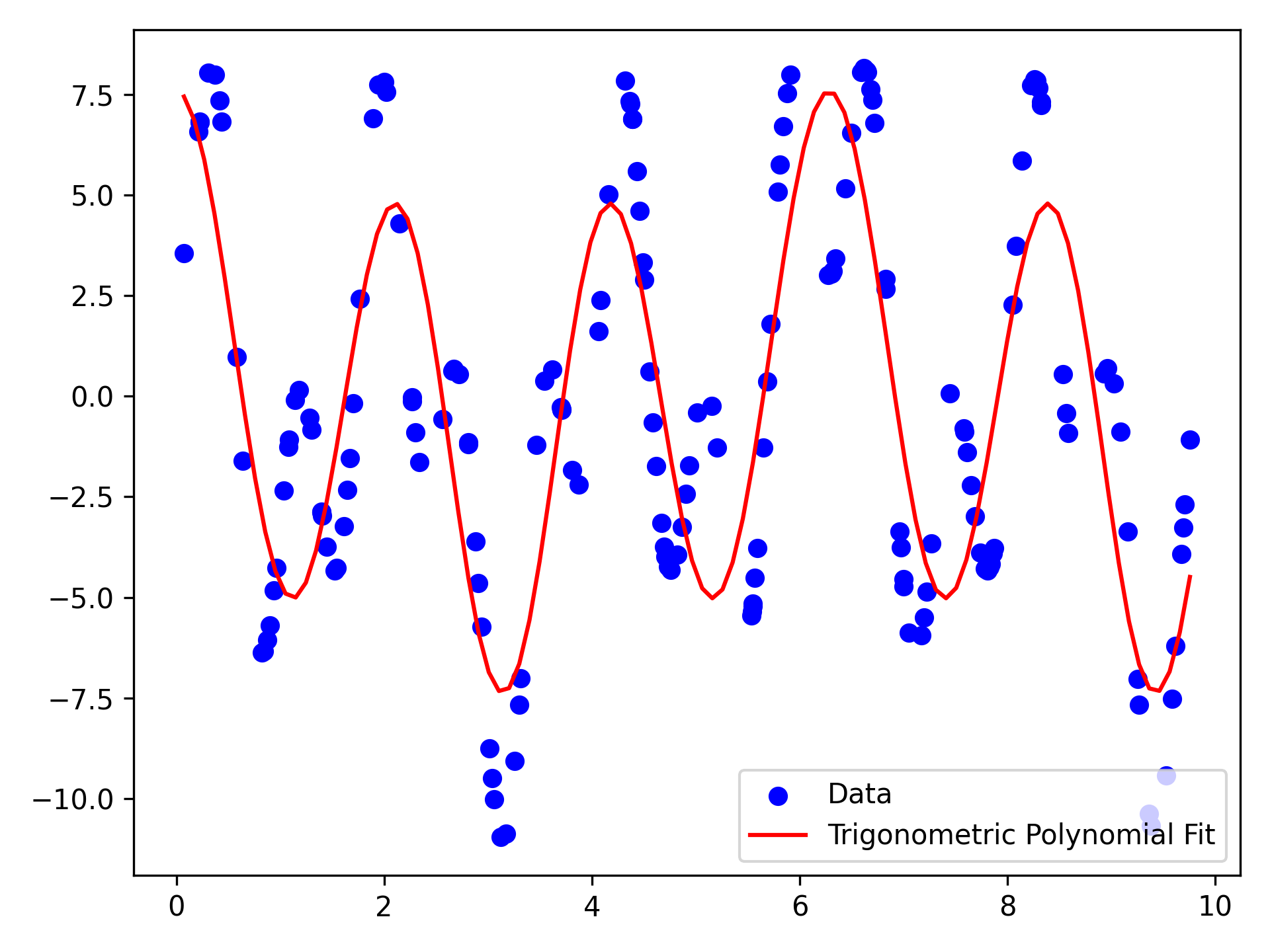
Trigonometric polynomials in \(L^2\)-spaces

API References: L2, SampleSpace, ProbabilityMeasure

fourier_polynomials.pyOutput

"""Fit a trigonometric polynomial to data using the L2 orthogonal projection operator."""

import matplotlib.pyplot as plt
import numpy as np

from sigalg.core import Index, RandomVector
from sigalg.l2 import L2

arr = np.load("data/fourier_data.npy")  # (1)!

component_names = Index().from_list(["X", "Y"])
Z = RandomVector(  # (2)!
    name="Z",
    index=component_names,
).from_numpy(array=arr)

Omega = Z.domain  # (3)!
P = Z.probability_measure

X, Y = Z.components  # (4)!

H = L2(sample_space=Omega, probability_measure=P)  # (5)!

_, u, _ = H.proj(  # (6)!
    rv=Y,
    subspace=[np.cos(n * X) for n in range(1, 5)],
)

x = np.linspace(X.data.min(), X.data.max(), 100)
y = sum(u[n - 1] * np.cos(n * x) for n in range(1, 5))  # (7)!

plt.scatter(X.data, Y.data, color="blue", label="Data")
plt.plot(x, y, color="red", label="Trigonometric Polynomial Fit")  # (8)!
plt.legend()
plt.tight_layout()
plt.show()

1. The data consists of \(175\) pairs \((x,y)\) of real numbers. We want to find a trigonometric polynomial that fits the data well.
2. Load the data into a RandomVector object using the from_numpy method.
3. The sample space \(\Omega\) and probability meausure \(P\) are automatically created; \(\Omega\) consists of the numbers \(0,1,\ldots,174\), and \(P\) is the uniform distribution on \(\Omega\).
4. Extract the component random variables \(X\) and \(Y\) from the random vector \(Z=(X,Y)\).
5. Create the \(L^2\)-space \(H = L^2(\Omega, \mathcal{F}, P)\), where \(\mathcal{F}\) is the default \(\sigma\)-algebra on \(\Omega\), the power set.
6. Perform an orthogonal projection of \(Y\) onto a subspace of trigonometric polynomials in \(X\). The coefficients of the best-fit polynomial are stored in a np.ndarray object u.
7. Extract the coefficients from u and create the best-fit polynomial.
8. Plot the data and the fitted polynomial.

Stochastic processes

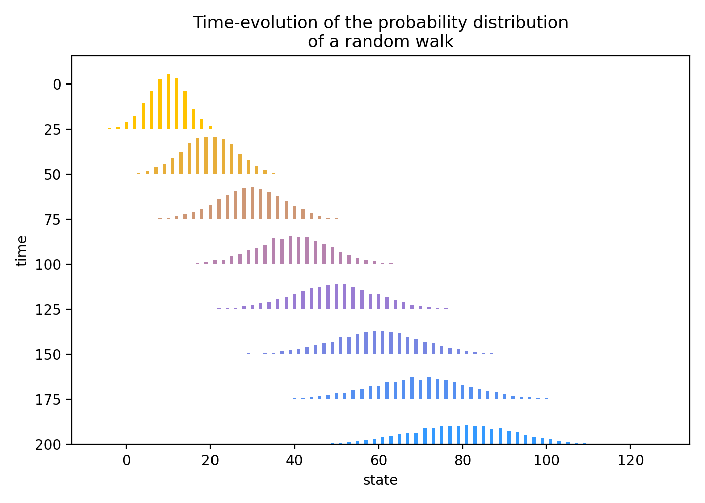
Diffusion of random walk transition probabilities

API References: Time, RandomWalk

random_walk_diffusion.pyOutput

"""Visualize the time-evolution of the transition probabilities of a random walk via a ridgeline plot, demonstrating a diffusion with positive drift."""

import matplotlib.pyplot as plt
from matplotlib.colors import LinearSegmentedColormap

from sigalg.core import Time
from sigalg.processes import RandomWalk

yellow = "#FFC300"
blue = "#3399FF"
purple = "#AA77CC"

T = Time.discrete(length=200)
X = RandomWalk(  # (1)!
    p=0.7,
    name="X",
    time=T,
).from_simulation(
    n_trajectories=10_000,
    random_state=42,
)

_, ax = plt.subplots(figsize=(7, 5))

n_plots = 8  # (2)!
time_step = 25
times = [time_step * k for k in range(1, n_plots + 1)]

cmap = LinearSegmentedColormap.from_list(  # (3)!
    "conditional_cmap", [yellow, purple, blue]
)
colors = [cmap(i / (n_plots - 1)) for i in range(n_plots)]

for color, t in zip(colors, times, strict=False):
    probabilities = X[t - 1].range.probability_measure.data  # (4)!
    probabilities.index = X[t - 1].range.data.values  # (5)!

    ax.bar(  # (6)!
        x=probabilities.index,
        height=-probabilities.values * 175,  # (7)!
        width=0.8,
        color=color,
        bottom=t,
    )

ax.invert_yaxis()
ax.set_xlabel("state")
ax.set_ylabel("time")
ax.set_title(
    "Time-evolution of the probability distribution\nof a random walk",
)
plt.tight_layout()
plt.show()

1. Simulate \(10{,}000\) trajectories of length \(200\) of a random walk \(X\) with initial state \(X_0=0\) and probability of an up-move \(p=0.7\).
2. Generate a list of times \(t=25, 50, \ldots, 200\) at which to plot the empirical probability distribution of \(X_t\).
3. Define custom colors.
4. The random variable \(X_t\) is simulated with draws \(\{x_1,x_2,\ldots,x_{10{,}000}\}\), where \(x_i\) is the value of the \(i\)-th trajectory at time \(t\). The probability distribution is uniform over these draws, \(P(\{x_i\}) = 1/10{,}000\) for \(i=1,2,\ldots,10{,}000\). The empirical probability distribution of \(X_t\) is computed by grouping the draws together and adding their uniform probabilities. So, if \(x\) is a value in the range of \(X_t\) and \(n_x\) is the number of draws equal to \(x\), then the empirical probability of \(X_t=x\) is \(P(X_t=x) = n_x/10{,}000\). This empirical probability distribution is first computed by accessing the range attribute, which groups the draws together, then accessing the data attribute of the probability_measure, which returns a pd.Series object containing the empirical probabilities of the unique values in the range of \(X_t\).
5. The data attribute of the range returns a pd.Series containing the unique values in the range of \(X_t\).
6. Plot an empirical probability distribution on a line of the ridgeline plot.
7. Scale the empirical probabilities by a factor of \(175\) to make the ridgeline plot easier to read.

Gambling strategy as an adapted process with winnings as an Itô integral

API References: RandomVariable, Time, ProcessTransforms, RandomWalk, StochasticProcess

gambling_strategy.pyOutput

"""Model a gambling strategy on a binary-outcome game as an adapted process."""

from sigalg.core import RandomVariable, Time
from sigalg.processes import ProcessTransforms, RandomWalk, StochasticProcess

T = Time.discrete(start=0, stop=3)  # (1)!

Y = RandomWalk(p=0.4, time=T, name="Y").from_enumeration()  # (2)!


def f0(Y: StochasticProcess) -> RandomVariable:  # (3)!
    return RandomVariable(domain=Y.domain).from_constant(1)


def f1(Y: StochasticProcess) -> RandomVariable:  # (4)!
    return 2 * (Y[1] > Y[0])


def f2(Y: StochasticProcess) -> RandomVariable:  # (5)!
    return 2 * (Y[2] > Y[1]) + 1 * (Y[1] > Y[0])


X = ProcessTransforms.transform(  # (6)!
    process=Y, functions=[f0, f1, f2], time=T[:-1]
).with_name("X")

winnings = X.ito_integral(Y)  # (7)!
expected_winnings = winnings.last_rv.expectation().item()  # (8)!

print("Is the game unfair to the bettor?", Y.is_supermartingale())  # (9)!
print("\nWhich games are winners and which are losers?\n", Y.increments())  # (10)!
print("\nBettor's strategy:\n", X)  # (11)!
print(
    "\nIs the bettor's strategy adapted?", X.is_adapted(Y.natural_filtration)
)  # (12)!
print("\nBettor's winnings:\n", winnings)  # (13)!
print(
    "\nIs the bettor's strategy a losing strategy?",
    winnings.is_supermartingale(Y.natural_filtration),
)  # (14)!
print("\nExpected winnings:", f"{expected_winnings:0.2f}")  # (15)!

1. Gameplay is indexed by the discrete time index \(T = \{0,1,2,3\}\), corresponding to three games played after the initial time \(0\).
2. The process \(Y\) is the price process of the game, which tracks the cumulative winnings of the bettor if they were to wager \(1\) unit on each game beginning from \(Y_0=0\). The (forward) increment \(\Delta Y_t = Y_{t+1} - Y_t\) represents the outcome of the \((t+1)\)-th game. An increment of \(+1\) represents a win for the bettor, and an increment of \(-1\) represents a loss. The probability of winning is \(p=0.4\), so the house has an edge.
3. A betting strategy is, by definition, a process \(X\) adapted to the natural filtration of \(Y\). The value \(X_t\) is the bettor's wager on the \((t+1)\)-th game. We construct such a process through three transformations \(X_0 = f_0(Y_0)\), \(X_1 = f_1(Y_0, Y_1)\), and \(X_2 = f_2(Y_0, Y_1, Y_2)\). We set \(f_0(Y_0)=1\), so the bettor wagers \(1\) unit on the first game, no matter what.
4. On the second game, the bettor wagers \(2\) units if the first game is a winner, and wagers nothing if the first game is a loser.
5. On the third game, the bettor wagers \(3\) units if the first two games are winners; wagers \(2\) units if the second game is a winner but the first game is a loser; wagers \(1\) unit if the first game is a winner but the second game is a loser; and wagers nothing if the first two games are losers.
6. Apply the transformations to the process \(Y\) to obtain \(X\).
7. The bettor's winnings are the Itô integral of \(X\) with respect to \(Y\).
8. Compute the expected winnings of the bettor after the three games.
9. Check that \(Y\) really is unfair to the bettor by verifying that \(Y\) is a supermartingale.
10. Print the increments of \(Y\) to see which games are winners and which are losers.
11. Print the betting strategy \(X\).
12. Check that \(X\) is adapted to the natural filtration of \(Y\).
13. Print the bettor's winnings.
14. Check if the bettor's strategy is a losing strategy by verifying if the winnings process is a supermartingale.
15. Print the expected winnings of the bettor after the three games.

Is the game unfair to the bettor? True

Which games are winners and which are losers?
 Stochastic process 'Y_increments':
time        0  1  2
trajectory         
0          -1 -1 -1
1          -1 -1  1
2          -1  1 -1
3          -1  1  1
4           1 -1 -1
5           1 -1  1
6           1  1 -1
7           1  1  1

Bettor's strategy:
 Stochastic process 'X':
time        0  1  2
trajectory         
0           1  0  0
1           1  0  0
2           1  0  2
3           1  0  2
4           1  2  1
5           1  2  1
6           1  2  3
7           1  2  3

Is the bettor's strategy adapted? True

Bettor's winnings:
 Stochastic process 'int X dY':
time        0  1  2  3
trajectory            
0           0 -1 -1 -1
1           0 -1 -1 -1
2           0 -1 -1 -3
3           0 -1 -1  1
4           0  1 -1 -2
5           0  1 -1  0
6           0  1  3  0
7           0  1  3  6

Is the bettor's strategy a losing strategy? True

Expected winnings: -0.60

Finance

Binomial asset pricing model

API References: BinomialPricingModel

binomial_pricing_model.pyText OutputFigures

"""Model the price process of a risky asset using a binomial tree."""

import matplotlib.pyplot as plt

from sigalg.core import Time
from sigalg.finance import BinomialPricingModel

S_0 = 100  # (1)!
u = 1.1  # (2)!
p = 0.7  # (3)!
r = 0.01  # (4)!
T = 3  # (5)!
time = Time.discrete(length=T)

S = BinomialPricingModel(  # (6)!
    initial_price=S_0,
    up_factor=u,
    up_prob=p,
    risk_free_rate=r,
    time=time,
)

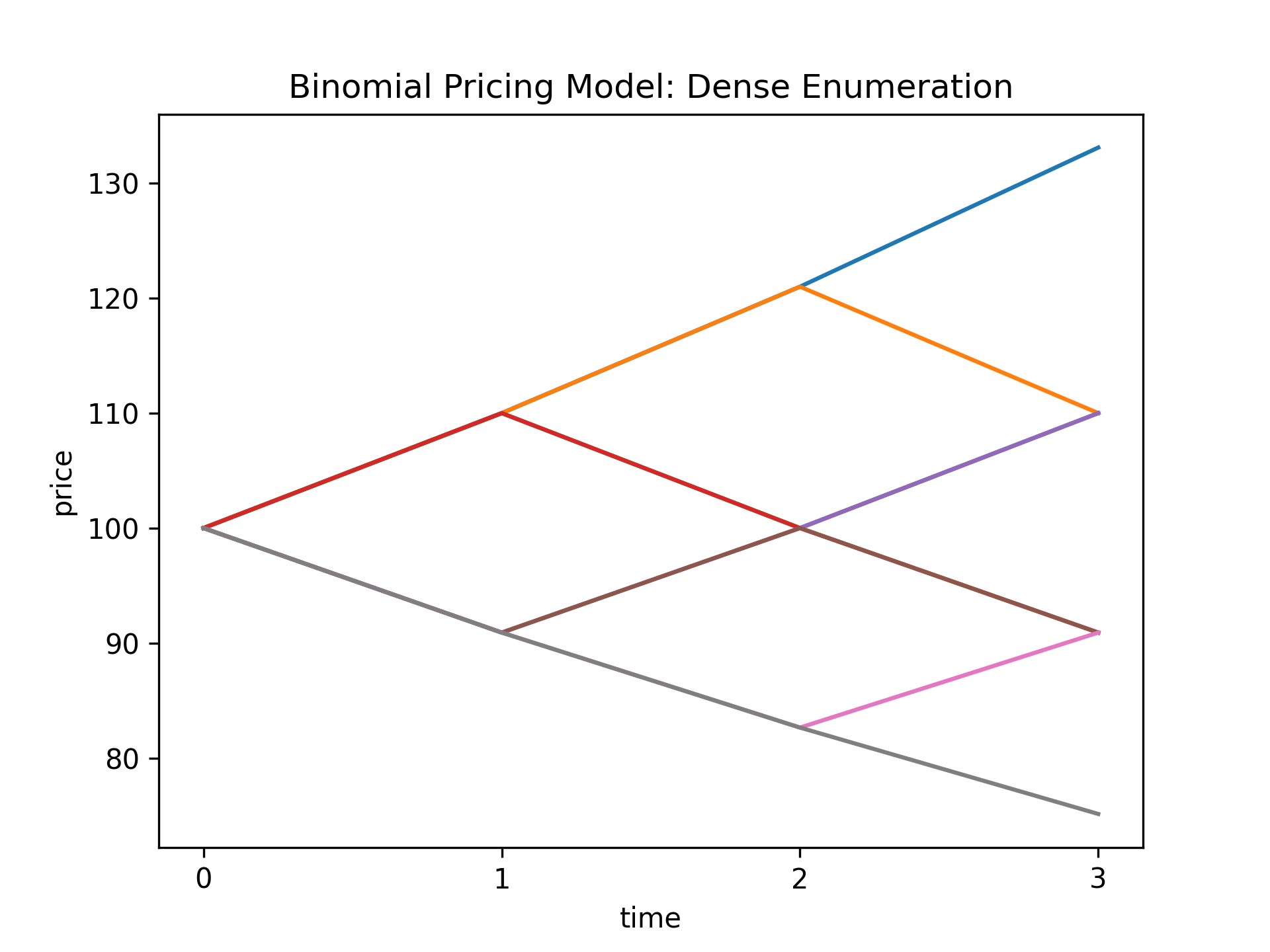
S.from_enumeration(enum_mode="dense")  # (7)!
print("Binomial Pricing Model (Dense Enumeration):\n", S)

S.plot_trajectories(  # (8)!
    y_label="price", title="Binomial Pricing Model: Dense Enumeration"
)
plt.show()

print(  # (9)!
    "\nReal-World Probability Measure (Dense Enumeration):\n", S.probability_measure
)
print("\nRisk Neutral Measure (Dense Enumeration):\n", S.risk_neutral_measure)  # (10)!

S_discounted = S.discount(rate=S.risk_free_rate)  # (11)!
print(
    "\nAre the discounted prices a martingale under the risk-neutral measure? ",
    S_discounted.is_martingale(probability_measure=S.risk_neutral_measure),
)

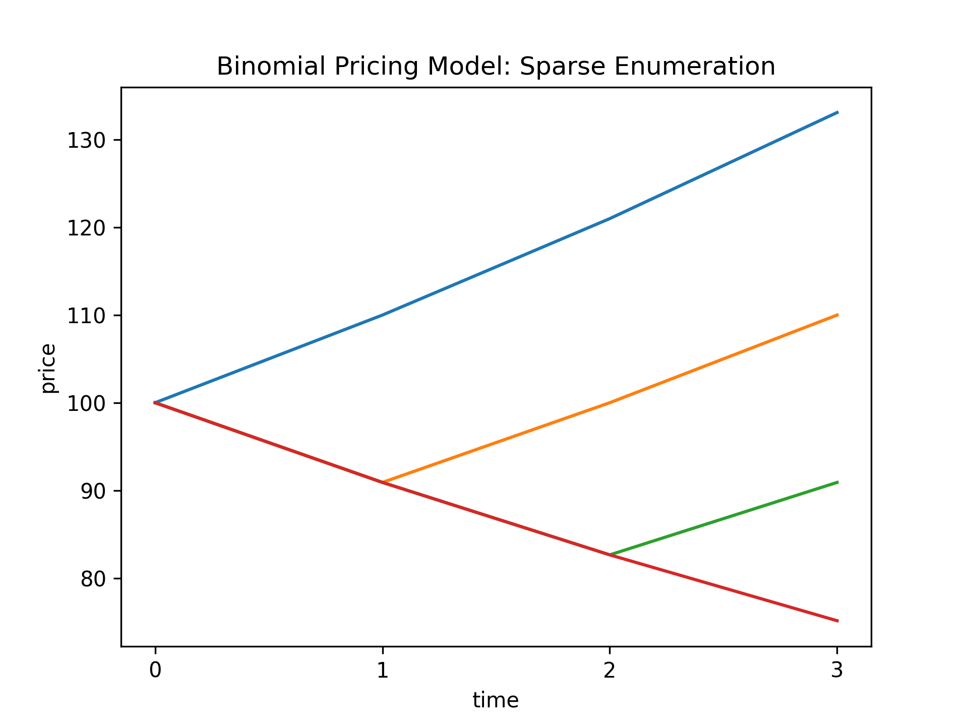
S.from_enumeration(enum_mode="sparse")  # (12)!
print("\nBinomial Pricing Model (Sparse Enumeration):\n", S)

S.plot_trajectories(  # (13)!
    y_label="price", title="Binomial Pricing Model: Sparse Enumeration"
)
plt.show()

print(  # (14)!
    "\nReal-World Probability Measure (Sparse Enumeration):\n", S.probability_measure
)
print("\nRisk Neutral Measure (Sparse Enumeration):\n", S.risk_neutral_measure)  # (15)!

1. The asset has an initial price of \(S_0=100\) USD.
2. For each time step in the model, the price of the asset can either increase by a factor of \(u=1.1\), or it can fall by a factor of \(d = 1/u \approx 0.91\).
3. The probability of an up-move is \(p=0.7\), and the probability of a down-move is \(1-p=0.3\).
4. The asset is traded in a market that includes a bank account with a risk-free per-period rate of interest \(r = 0.01\).
5. The length of the model is \(3\) time steps.
6. Set up the binomial pricing model with the parameters defined above.
7. The from_enumeration method in dense mode computes all \(8=2^3\) possible price trajectories of the asset.
8. Plot all the price trajectories of the asset in the dense enumeration.
9. The real-world probability measure is computed from the up-move probability \(p\) and down-move probability \(1-p\).
10. The risk-neutral measure is computed from the risk-free rate \(r\) and the up and down factors \(u\) and \(d\).
11. Check that the discounted price process is a martingale under the risk-neutral measure.
12. The from_enumeration method in sparse mode computes four canonical price trajectories of the asset.
13. Plot the four canonical price trajectories of the asset in the sparse enumeration.
14. The real-world probability measure is computed from the up-move probability \(p\) and down-move probability \(1-p\).
15. The risk-neutral measure is computed from the risk-free rate \(r\) and the up and down factors \(u\) and \(d\).

Binomial Pricing Model (Dense Enumeration):
 Stochastic process 'S':
time          0           1           2           3
trajectory                                         
0           100  110.000000  121.000000  133.100000
1           100  110.000000  121.000000  110.000000
2           100  110.000000  100.000000  110.000000
3           100  110.000000  100.000000   90.909091
4           100   90.909091  100.000000  110.000000
5           100   90.909091  100.000000   90.909091
6           100   90.909091   82.644628   90.909091
7           100   90.909091   82.644628   75.131480

Real-World Probability Measure (Dense Enumeration):
 Probability measure 'P':
            probability
trajectory             
0                 0.343
1                 0.147
2                 0.147
3                 0.063
4                 0.147
5                 0.063
6                 0.063
7                 0.027

Risk Neutral Measure (Dense Enumeration):
 Probability measure 'Q':
            probability
trajectory             
0              0.147676
1              0.131711
2              0.131711
3              0.117472
4              0.131711
5              0.117472
6              0.117472
7              0.104773

Are the discounted prices a martingale under the risk-neutral measure?  True

Binomial Pricing Model (Sparse Enumeration):
 Stochastic process 'S':
time            0           1           2           3
trajectory                                           
0           100.0  110.000000  121.000000  133.100000
1           100.0   90.909091  100.000000  110.000000
2           100.0   90.909091   82.644628   90.909091
3           100.0   90.909091   82.644628   75.131480

Real-World Probability Measure (Sparse Enumeration):
 Probability measure 'P':
            probability
trajectory             
0                 0.343
1                 0.441
2                 0.189
3                 0.027

Risk Neutral Measure (Sparse Enumeration):
 Probability measure 'Q':
            probability
trajectory             
0              0.147676
1              0.395134
2              0.352417
3              0.104773