Introducing SigAlg: Measure-Theoretic Probability in Python
Stochastic processes
IID processes
Random walks
Probability theory
Sigma-algebras
Information theory
SigAlg
SciPy
Python
Published
February 3, 2026
Introduction
For the past four-ish months, I’ve been working on a Python library called SigAlg (named after a \(\sigma\)-algebra, duh), designed to provide mathematically faithful implementations of measure-theoretic probability. I’ve recently made early versions available on PyPI, made the GitHub repo public, and put up a documentation site that is around 90% done. I’m still very much in the early stages of development, but if I keep obsessing over perfection, it’ll never be released. So it’s time to kick this baby bird out of the nest and hope it doesn’t fall to its death.
Where did this thing come from?
I have recently taken a liking to mathematical finance. (To the extent that I now listen to finance-oriented podcasts and pay some attention to the markets. I know—as a recovering pure mathematician, I feel gross just saying that. No offense finance people.) The issue is, that I come from a very different mathematical upbringing, so I knew next to nothing about the deeper parts of stochastic process theory, stochastic calculus, and all that stuff. So, as I’m grinding my way through some textbooks playing catch-up, I found myself wanting to experiment with code, but I couldn’t find any libraries that implemented the concepts in a way that felt natural and mathematically faithful. There’s a really big jump between, say, a \(\sigma\)-algebra that you manipulate in your head and push around on a sheet of paper, and the code that implements it using existing Python libraries. Sure, you can perform a group_by on a pd.DataFrame that will partition your “sample space” into the “atoms” of your \(\sigma\)-algebra, but I wanted a semantically meaningful API that feels like you’re writing mathematics on paper. That leads us here. I give you SigAlg.
I will introduce you to SigAlg in this post, which is mostly an extended version of the random walk example on the landing page of the documentation site. Future blog posts will cover more advanced topics.
Generalities on stochastic processes
First, before any code, let’s make sure we agree on definitions and terminology. Allow me to put on my math professor hat.
Given a nonempty set \(T\subset \mathbb{R}\), our definition of a stochastic process requires us to consider the function space \(\mathbb{R}^T\), which consists of all \(\mathbb{R}\)-valued functions on \(T\).
Definition 1 Let \(\Omega\) be a probability space and let \(T\subset \mathbb{R}\) be a nonempty subset. A stochastic process, with index set \(T\), is a function
\[
X: \Omega \to U
\]
where \(U\) is a subset of the function space \(\mathbb{R}^T\). We require \(X\) be such that, for each \(t \in T\), the function \[
X_t : \Omega \to \mathbb{R}, \quad \omega \mapsto X(\omega)(t),
\]
is a random variable on \(\Omega\).
The requirement that “\(X_t\) is a random variable” means that \(X_t\) is a measurable function with respect to the Borel algebra on \(\mathbb{R}\) and the given \(\sigma\)-algebra on \(\Omega\). If this makes sense, then good—if not, the reader can simply ignore this technical detail.
The index set \(T\) is often conceptualized as time, and when \(T\) is countable we say that \(X\) is a discrete-time stochastic process, while when \(T\) is an interval in \(\mathbb{R}\) (or \(\mathbb{R}\) itself) we say that \(X\) is a continuous-time stochastic process. Similarly, if each random variable \(X_t\) is discrete, we say that \(X\) is a discrete-state stochastic process, while if each \(X_t\) is continuous, we say that \(X\) is a continuous-state stochastic process.
Note that a stochastic process \(X\) and the collection of random variables \(\{X_t\}_{t\in T}\) that it determines are equivalent objects. To be more precise, note that obviously \(X\) determines each random variable \(X_t\), but conversely, given a collection of random variables \(\{X_t\}_{t\in T}\), we can construct a stochastic process \(X\) via the formula
is called a trajectory (or sample path) of the stochastic process. It is these trajectories that are often the central objects of study in applications of stochastic processes.
Technically, in order for the law of \(X\) to be well-defined, \(X\) needs to be a measurable function with respect to a \(\sigma\)-algebra on \(U\). This is indeed the case. See, for example, Lemma 4.1 in [1].
If \(X: \Omega \to U\) is a random variable as in the definition above, and if \(P\) is the probability measure on \(\Omega\), then \(X\) has a well-defined law, which is a probability measure \(P_X\) on \(U\) given by
for all measurable sets \(A \subset U\). It is an important fact (see Proposition 4.2 in [1]) that this law is uniquely determined by the finite-dimensional distributions of \(X\), which are the probability measures on \(\mathbb{R}^n\) of the form
where \(n\) ranges over all positive integers, \(t_1, \ldots, t_n\) range over all indices in \(T\), and \(B\subset \mathbb{R}^n\) is a Borel set. Note that these are the laws of the random vectors
Specializing this fact, in the case of a finite index set \(T = \{t_1, \ldots, t_n\}\), we conclude that the law (1) of \(X\) is completely determined by the (single!) random vector \((X_{t_1}, \ldots, X_{t_n})\), since all the other finite-dimensional distributions can be obtained by marginalizing the law of this one.
Independent and identically distributed processes
After all the generalities and abstractions in the previous section, we now bring everything down to earth and discuss what might be the simplest examples of stochastic processes:
Definition 2 Let \(X:\Omega \to U \subset \mathbb{R}^T\) be a \(T\)-indexed stochastic process on a probability space \(\Omega\). Then \(X\) is called an independent and identically distributed (IID) process if the random variables \(\{X_t\}_{t\in T}\) are independent and identically distributed.
The finite-dimensional distributions of an IID process are given by the formula
where we assume \(B = B_1 \times \cdots \times B_n \subset \mathbb{R}^n\) is a product of Borel sets.
A simple example of an IID process is a sequence of Bernoulli random variables indexed by a finite set \(T = \{1,2,\ldots,n\}\), which can be used to model a sequence of \(n\) coin flips where \(X_t = 1\) represents heads and \(X_t = 0\) represents tails on the \(t\)-th flip. Such a process can be implemented using the SigAlg library and its interface with SciPy:
In constructing the Time instance T modeling the index set \(T = \{1,2,3\}\), note that the length parameter is 2, which is the length of time spanned by the interval from 1 to 3. In particular, the length parameter is not the length in the sense of the Python magic method len(), which would return the number of time points, 3.
from scipy.stats import bernoullifrom sigalg.core import Timefrom sigalg.processes import IIDProcess# Construct time index [1, 2, 3]. See the aside in the margin --->T = Time.discrete(start=1, length=2)# Set the parameters for the IID processX = IIDProcess( distribution=bernoulli(p=0.7), support=[0, 1], time=T,)# Generate all possible trajectoriesX.from_enumeration()print(X)
The printout shows an IID process \(X\) on the index set \(T = \{1,2,3\}\), where each \(X_t\sim \mathcal{B}er(0.7)\) is a Bernoulli random variable with parameter \(p=0.7\). The three time-indexed columns correspond to the values of the three random variables \(X_1, X_2, X_3\). SigAlg models the domain \(\Omega\) as the trajectory indices, so \(\Omega = \{0,1,\ldots,7\}\). This may be verified by checking the domain attribute of our process:
print(X.domain)
Sample space 'Omega':
[0, 1, 2, 3, 4, 5, 6, 7]
Thus, the rows of the printout may be conceptualized as the trajectories
as \(\omega\) ranges over the domain \(\Omega = \{0,1,\ldots,7\}\). Since each \(X_t\) has only two possible outcomes, the entire process has \(2^3 = 8\) possible trajectories, all being listed in the printout.
Each trajectory of the process has a probability computed via the formula (2) above. For example, for the trajectory \(X(3)=(0,1,1)\) we have
The probabilities of each trajectory can be accessed via the probability_measure attribute of the process. In this printout, note that trajectory 3 does indeed have the correct probability:
Technically, the domain \(\Omega\) is supposed to have a \(\sigma\)-algebra with respect to which the process \(X\) is measurable, but this is not enforced in SigAlg. However, \(\Omega\) does have the natural filtration induced by \(X\), which is modeled in SigAlg. In our case, this filtration is a nested sequence of \(\sigma\)-algebras
In general, a containment \(\mathcal{F}\subset \mathcal{G}\) of \(\sigma\)-algebras on a common (finite!) sample space \(\Omega\) is equivalent to the statement that every atom of \(\mathcal{F}\) is a union of atoms of \(\mathcal{G}\), which, in turn, is the same as saying that every atom of \(\mathcal{G}\) is a subset of some atom of \(\mathcal{F}\). In the present case, the reader will see this relationship in the “information flow” diagram below.
is the \(\sigma\)-algebra generated by the random vector \((X_1, X_2, \ldots, X_t)\). This is the coarest \(\sigma\)-algebra with respect to which \(X_1, X_2, \ldots, X_t\) are all measurable. But, since \(\Omega\) is finite, \(\sigma\)-algebras can be completely described in terms of their atoms, which are the minimal non-empty sets in the \(\sigma\)-algebra (and which partition \(\Omega\)). The atoms of the \(\sigma\)-algebra \(\mathcal{F}_t\) are simply the level sets of the random vector \((X_1,X_2,\ldots,X_t)\) as a function on \(\Omega\).
In SigAlg, \(\sigma\)-algebras are stored internally by associating to each sample point \(\omega\in \Omega\) an atom identifier that specifies which atom the sample point belongs to. Since the atoms of the \(\sigma\)-algebras \(\mathcal{F}_t\) are the level sets of \((X_1,X_2,\ldots,X_t)\), a convenient set of atom IDs are the values of these random vectors themselves.
For example, here are the atom IDs of \(\mathcal{F}_1\):
import pandas as pd# Get the natural filtrationF = X.natural_filtration# Grab the F1 sigma-algebraF1 = F[1]# Display the atom IDs alongside the process data.# Almost all objects in SigAlg have `data` attributes that return Pandas objects.display_df = pd.concat([X.data, F1.data.rename("F1 atom ID")], axis=1)print(display_df)
Indeed, notice that the atom IDs are simply the values of the random variable \(X_1(\omega)\in \{0,1\}\), as \(\omega\) ranges over \(\Omega = \{0,1,\ldots,7\}\).
Here are the atom IDs of \(\mathcal{F}_2\):
F2 = F[2]display_df = pd.concat([display_df, F2.data.rename("F2 atom ID")], axis=1)print(display_df)
In this last case, note that each \(\omega\) has its own unique atom ID, which means that the \(\sigma\)-algebra \(\mathcal{F}_3\) is the power set on \(\Omega\), i.e., the finest \(\sigma\)-algebra on \(\Omega\).
In probability theory, these filtrations (increasing sequences of \(\sigma\)-algebras) are intended to model “refinements of information” available to an observer over time. For our current IID process \(X\), the natural filtration might have the following concrete information-theoretic interpretation: Suppose that each \(X_t\) (for \(t=1,2,3\)) does indeed model the outcome of a (biased) coin flip, with \(X_t=0\) representing a tail, and \(X_t=1\) a head on the \(t\)-th flip. Now, suppose that all three flips have occured, so that a definite trajectory \(X(\omega)\) of the process has been identified, which is the same as saying that a definite sample point \(\omega\) has been identified, since the sample points and their trajectories are in one-to-one correspondence.
However, suppose that our observer does not yet know which \(\omega\) has been realized, and its true value is only progressively revealed over time, flip by flip.
At time \(t=1\), the observer sees the result of the first flip, \(X_1(\omega)\). With this information, the observer would be able to identify which of the two atoms of \(\mathcal{F}_1\) contains the sample point \(\omega\). And conversely, if the observer knew which of these atoms contained \(\omega\), then the observer would also know the value of \(X_1(\omega)\). So, in this sense, the information contained in knowledge of the value \(X_1(\omega)\) is equally well contained in the \(\sigma\)-algebra \(\mathcal{F}_1\).
Note that while this information reduces some uncertainty about the identity of \(\omega\), it does not reduce all of it. For within each atom of \(\mathcal{F}_1\), the differenent trajectories \(X(\omega)\) are indistinguishable, given only the information in \(\mathcal{F}_1\).
Now, at time \(t=2\), the observer sees the result of the second flip, \(X_2(\omega)\). With this additional information, combined with knowledge of the first flip, the observer would be able to identify which of the four atoms of \(\mathcal{F}_2\) contains the sample point \(\omega\). But again, while this reduces more of the uncertainty about \(\omega\), it does not eliminate it entirely, for the observer still cannot distinguish between the trajectories \(X(\omega)\) within each of the four atoms of \(\mathcal{F}_2\), given only the information in \(\mathcal{F}_2\).
Finally, at time \(t=3\), the observer sees the result of the third flip, \(X_3(\omega)\). As in the previous two cases, with this new information, the observer can identify which of the eight atoms of \(\mathcal{F}_3\) contains the sample point \(\omega\). But since \(\mathcal{F}_3\) is the power set, this amounts to complete information on \(\omega\). The trajectory \(X(\omega)\) is now fully determined.
This “flow” of information, refining the observer’s knowledge over time, is precisely what a filtration models. This flow can be visualized through SigAlg’s interface with Plotly, to create a Sankey-style figure:
# These two lines are only necessary to render in Quarto markdown.# The reader may remove them.import plotly.io as piopio.renderers.default ="plotly_mimetype+notebook_connected"from sigalg.core import plot_information_flow# Reusable plotting parametersplot_config =dict( height=400, node_color="#FFC300", font_color="#FAF9F6", link_color="rgba(168, 165, 159, 0.5)", background_color="#121212", font_family="monospace",)fig = plot_information_flow( filtration=F, title="Natural filtration of 'X'", show_atom_counts=False,**plot_config,)fig.show()
As we read the figure from left to right through time, notice that each atom is split into a union of atoms in the next \(\sigma\)-algebra. This illustrates how the observer’s knowledge is refined over time as more information becomes available. If earlier atoms were not unions of later atoms, then one of the containments \(\mathcal{F}_1 \subset \mathcal{F}_2\) or \(\mathcal{F}_2 \subset \mathcal{F}_3\) would be violated, which means that the three \(\sigma\)-algebras would not form a filtration. (Recall the most recent margin note above.)
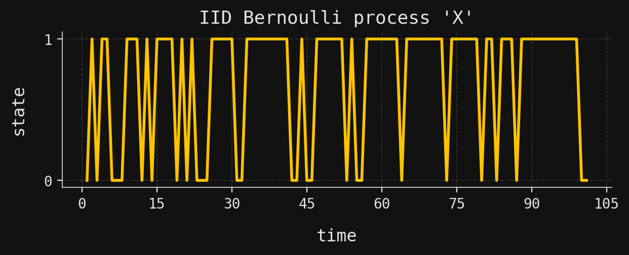
The trajectories of our process \(X\) are short. Longer trajectories can be generated by increasing the length parameter in the Time instance, though care must be taken since the number of possible trajectories grows exponentially with the length of the trajectories. For long trajectories, it is often more practical to work with Monte Carlo simulations rather than exhaustive enumerations. In the next code block, we simulate a single trajectory of length 100 from the same IID Bernoulli process above and plot it:
import matplotlib.pyplot as plt# The reader may remove this line, or set their own custom styleplt.style.use("../../aux-files/custom-theme.mplstyle")# Set the time index of the process to a longer lengthT = Time.discrete(start=1, length=100)X.time = T# Simulate a single trajectoryX.from_simulation( n_trajectories=1, random_state=42,)# Plot the trajectory_, ax = plt.subplots(figsize=(7, 2))X.plot_trajectories(ax=ax)plt.show()
The trajectory is plotted by first plotting the points \((t, X_t)\) for each time \(t=1,2,\ldots,101\), and then connecting these points with lines for visual clarity.
Random walks
With IID processes as building blocks, we can construct more complex stochastic processes such as random walks.
Definition 3 Let \(p\) be a real number with \(0\leq p \leq 1\), let \(x_0\) and \(t_0\) be integers, and let
\[
T = \{t_0, t_0+1, t_0+2, \ldots, t_0 + n\},
\]
where \(n\) is either a positive integer or \(\infty\). Then a random walk of length \(n\), with initial position \(x_0\) and initial time \(t_0\), is a stochastic process \(X\) with the following properties:
We have \(X_{t_0}=x_0\), the constant random variable.
The increments\[
\Delta X_t \stackrel{\text{def}}{=} X_t - X_{t-1}, \quad t \in T, \ t\neq t_0,
\] are IID random variables.
Each increment \(\Delta X_t\) takes either the value \(1\) or \(-1\), the former with probability \(p\) and the latter with probability \(q=1-p\).
When \(p\neq 0.5\), the random walk is said to have drift, which we will discuss in more detail below. If \(p=0.5\), the random walk is said to be symmetric.
The reason for the name “random walk” is that each trajectory \(X(\omega)\) can be visualized as a path on the integer number line starting at \(x_0\), where at each discrete time \(t\) a step is taken that moves either one unit to the right (when \(\Delta X_t=1\), with probability \(p\)) or one unit to the left (when \(\Delta X_t=-1\), with probability \(q\)). Over many steps, this results in a “wandering” behavior that resembles a random walk. The random variable \(X_t\) represents the position of the walk after \(t\) steps.
The SigAlg library provides the RandomWalk class to model these processes, but it is instructive to build a random walk from scratch using the IID processes in the previous section. To do this, note that each \(X_t\) is the cumulative sum of the increments up to time \(t\), plus the initial state \(X_{t_0} = x_0\):
Notice the formal similarity between this equation and the the Fundamental Theorem of Calculus: \[f(t) = f(t_0) + \int_{t_0}^tdf(s),\] where we write \(df(s) = f'(s) \, ds\).
Thus, by modeling the increments \(\Delta X_t\) in SigAlg as an IID process, we can model a random walk \(X\) as the cumulative sum of these increments plus the starting point \(x_0\).
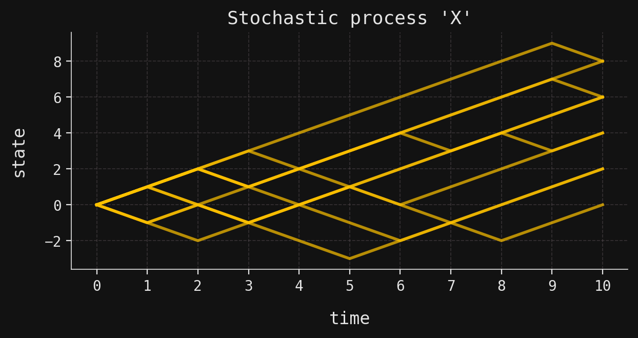
To begin, let’s suppose we want to model a random walk of length \(n=10\), with initial position \(x_0=0\), with initial time \(t_0=0\), and with probability \(p=0.7\) of stepping “to the right.” Then, note that
\[
\Delta X_t = 2B_t -1
\]
for \(1 \leq t \leq 10\), where \(B_t \sim \mathcal{B}er(0.7)\). Thus, in SigAlg, we write:
from sigalg.core import RandomVariable# The increments start at time t=1 and stop at t=10T = Time.discrete(start=1, stop=10)# Define the IID Bernoulli processB = IIDProcess( distribution=bernoulli(p=0.7), time=T, name="B",).from_simulation( n_trajectories=10, random_state=42,)# Construct the increment processDelta_X =2* B -1# Construct the random walk process by cumulative summationX = Delta_X.cumsum().with_name("X")# Insert the initial stateX.insert_rv(state=0, time=0, in_place=True)print(X)
We have simulated ten trajectories of the random walk. We see that the final position of trajectory 3 is 6, while the final position of trajectory 9 is 8. A plot of these simulated trajectories is shown below:
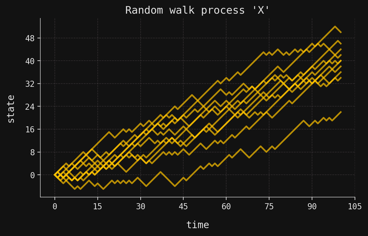
Longer trajectories reveal the “drift” that we mentioned above. To make these longer trajectories, we use the built-in RandomWalk class in SigAlg, which (essentially) internally implements the same construction as above. The following code simulates ten trajectories of length 100 with the same parameters as our original random walk: