What is information theory?

Introduction

Blah blah blah blah blah blah blah blah blah blah blah blah blah blah blah blah blah blah blah blah blah blah blah blah blah blah blah blah blah blah blah blah blah blah blah blah blah blah blah blah blah blah blah blah blah blah blah blah blah blah blah blah blah blah blah blah.

n = 6
xs = range(1, n+1)
fxs = poisson.pmf(xs, mu=3)
fxs /= fxs.sum()

def fy(y):
  return sum([beta.pdf(y, a=x, b=3) * fx for x, fx in zip(xs, fxs)])

fig = plt.figure(figsize=(8, 8))
gs = gridspec.GridSpec(2, 2, height_ratios=[1, 2])

ax1 = fig.add_subplot(gs[0, 0])
ax1.bar(xs, fxs, width=0.4, zorder=2)
ax1.set_xlabel(r"hours studied ($x$)")
ax1.set_ylabel("probability")
ax1.set_title(r"marginal mass $f(x)$")
ax1.set_xticks(range(1, 7))

grid = np.linspace(0, 1, num=250)
ax2 = fig.add_subplot(gs[0,1])
ax2.plot(grid, fy(grid))
ax2.fill_between(grid, fy(grid), zorder=2, alpha=0.1)
ax2.xaxis.set_major_formatter(PercentFormatter(xmax=1))
ax2.set_title(r"marginal density $f(y)$")
ax2.set_xlabel("test score ($y$)")
ax2.set_ylabel("probability density")

conditional_colors = [conditional_cmap(i/(n-1)) for i in range(n)]
ax3 = fig.add_subplot(gs[1,:])
for x, fx in zip(xs, fxs):
    joint_vals = 1.7 * beta.pdf(x=grid, a=x, b=3) * fx
    ax3.fill_between(grid, x, x + joint_vals, color=conditional_colors[x-1], zorder=2, alpha=0.1)
    ax3.plot(grid, x + joint_vals, color=conditional_colors[x-1], zorder=2)
ax3.set_ylabel(r"hours studied ($x$)")
ax3.set_xlabel(r"test score ($y$)")
ax3.xaxis.set_major_formatter(PercentFormatter(xmax=1))
ax3.set_title(r"joint mass/density $f(x,y)$")

plt.tight_layout()
plt.subplots_adjust(wspace=0.4, hspace=0.4)
plt.show()

_, ax = plt.subplots(figsize=(6, 4))

for x in xs:
  ax.plot(grid, beta.pdf(x=grid, a=x, b=3), color=conditional_colors[x-1], label=x)
ax.legend(title=r"hours studied ($x$)", loc="center left", bbox_to_anchor=(1, .5))
ax.xaxis.set_major_formatter(PercentFormatter(xmax=1))
ax.set_title(r"conditional densities $f(y|x)$")

ax.set_xlabel(r"test score ($y$)")
ax.set_ylabel("probability density")

plt.tight_layout()
plt.show()

Y_entropy, _ = quad(lambda y: -fy(y) * np.log(fy(y)), 0, 1)
Y_entropy - sum([beta.entropy(a=x, b=3) * fx for x, fx in zip(xs, fxs)])

0.20054350545969515

Basic definitions

Definition 1 Let \(X\) and \(Y\) be two random variables with density functions \(f(x)\) and \(f(y)\), respectively.

1. The surprisal of an observed value \(X=x\) is the quantity \[ I(x) = -\log{f(x)}, \] where the logarithm is the natural one.

2. The conditional surprisal of an observed value \(Y=y\), given \(X=x\), is the quantity \[ I(y|x) = -\log{f(y|x)}. \]

Definition 2 Let \(X\) and \(Y\) be two random variables with density functions \(f(x)\) and \(f(y)\), respectively.

1. The entropy of \(X\) is the quantity \[ H(X) = E_{x\sim f(x)}(I(x)). \]

2. The conditional entropy of \(Y\), given an observed value \(X=x\), is the quantity

\[ H(Y\mid X=x) = E_{y\sim f(y|x)}(I(y\mid x)). \]

3. The conditional entropy of \(Y\), given \(X\), is the quantity

\[ H(Y\mid X) = E_{x\sim f(x)}(H(Y\mid X=x)). \]

Mutual information of jointly discrete random variables

n = 6
fxy = np.random.rand(n ** 2)
fxy /= fxy.sum()
fxy = fxy.reshape(n, n)

fx = fxy.sum(axis=1)
fy = fxy.sum(axis=0)

fig = plt.figure(figsize=(8, 8))
gs = gridspec.GridSpec(2, 2, height_ratios=[1, 1.5])

ax1 = fig.add_subplot(gs[0, 0])
ax1.bar(range(n), fx, width=0.4, zorder=2)
ax1.set_xlabel(r"$x$")
ax1.set_ylabel("probability")
ax1.set_title(r"marginal distribution $f(x)$")

ax2 = fig.add_subplot(gs[0, 1], sharex=ax1, sharey=ax1)
ax2.bar(range(n), fy, width=0.4, zorder=2)
ax2.set_xlabel(r"$y$")
ax2.set_ylabel("probability")
ax2.set_title(r"marginal distribution $f(y)$")

ax3 = fig.add_subplot(gs[1,:])
sns.heatmap(fxy.T, annot=True, fmt=".3f", cmap=heatmap_cmap, linewidth=8, linecolor=grey, zorder=2, cbar_kws={'label': 'probability'}, ax=ax3)
ax3.invert_yaxis()
ax3.set_xlabel(r"$x$")
ax3.set_ylabel(r"$y$")
ax3.set_title(r"joint distribution $f(x,y)$")

plt.tight_layout()
plt.subplots_adjust(wspace=0.4, hspace=0.4)
plt.show()

fig, axes = plt.subplots(nrows=2, ncols=3, sharey=True, sharex=True)
conditionals = []

for x, ax in enumerate(axes.flatten()):
  f_y_given_x = fxy[x, :] / fxy[x, :].sum()
  conditionals.append(f_y_given_x)
  ax.bar(range(n), f_y_given_x, width=0.4, zorder=2)
  ax.set_xticks(range(n))  
  ax.set_xticklabels(range(n))
  ax.set_title(rf"$x={x}$")
  
fig.supxlabel(r"$y$")
fig.supylabel("probability")
fig.suptitle(r"conditional distributions $f(y\mid x)$")

plt.tight_layout()
plt.subplots_adjust(hspace=0.8)
plt.show()

info = entropy(fy) - sum([entropy(f_y_given_x) * fx[x] for x, f_y_given_x in enumerate(conditionals)])
print(f"The mutual information is I(X,Y) = {info:.4f}.")

The mutual information is I(X,Y) = 0.2032.

Mutual information of jointly normal random variables

Theorem 1 Let \((X,Y) \sim \mathcal{N}_2(\boldsymbol{\mu}, \boldsymbol{\Sigma})\) be a \(2\)-dimensional normal random vector with

\[ \boldsymbol{\mu}^\intercal = \begin{bmatrix} \mu_X & \mu_Y \end{bmatrix} \quad \text{and} \quad \boldsymbol{\Sigma}= \begin{bmatrix} \sigma_X^2 & \rho \sigma_X \sigma_Y \\ \rho \sigma_X \sigma_Y & \sigma_Y^2 \end{bmatrix}, \]

where \(X \sim \mathcal{N}(\mu_X,\sigma_X^2)\), \(Y\sim \mathcal{N}(\mu_Y,\sigma_Y^2)\), and \(\rho\) is the correlation between \(X\) and \(Y\). Then

\[ (Y \mid X=x) \sim \mathcal{N}\left(\mu_Y + (x-\mu_X) \frac{\rho \sigma_Y}{\sigma_X}, \ \sigma_Y^2(1-\rho^2) \right) \]

for all \(x\).

def plot_multivar(ax, muX, muY, sigmaX, sigmaY, x, y, labels=False):
  Sigma = np.array([[sigmaX ** 2, rho * sigmaX * sigmaY], [rho * sigmaX * sigmaY, sigmaY ** 2]])
  Mu = np.array([muX, muY])
  U = multivariate_normal(mean=Mu, cov=Sigma)
  grid = np.dstack((x, y))
  z = U.pdf(grid)
  contour = ax.contour(x, y, z, colors=yellow, alpha=0.5)
  if labels:
    ax.clabel(contour, inline=True, fontsize=8)
  
def plot_conditional(ax, muX, muY, sigmaX, sigmaY, rho, y, x_obs):
  mu = muY + (x_obs - muX) * rho * sigmaY / sigmaX
  sigma = sigmaY * np.sqrt(1 - rho ** 2)
  x = norm(loc=mu, scale=sigma).pdf(y)
  ax.plot(-x + x_obs, y, color=blue)
  ax.fill_betweenx(y, -x + x_obs, x_obs, color=blue, alpha=0.4)

def plot_combined(ax, muX, muY, sigmaX, sigmaY, rho, x, y, x_obs, labels=False):
  plot_multivar(ax, muX, muY, sigmaX, sigmaY, x, y, labels)
  y = np.linspace(np.min(y), np.max(y), num=250)
  plot_conditional(ax, muX, muY, sigmaX, sigmaY, rho, y, x_obs[0])
  plot_conditional(ax, muX, muY, sigmaX, sigmaY, rho, y, x_obs[1])
  plot_conditional(ax, muX, muY, sigmaX, sigmaY, rho, y, x_obs[2])
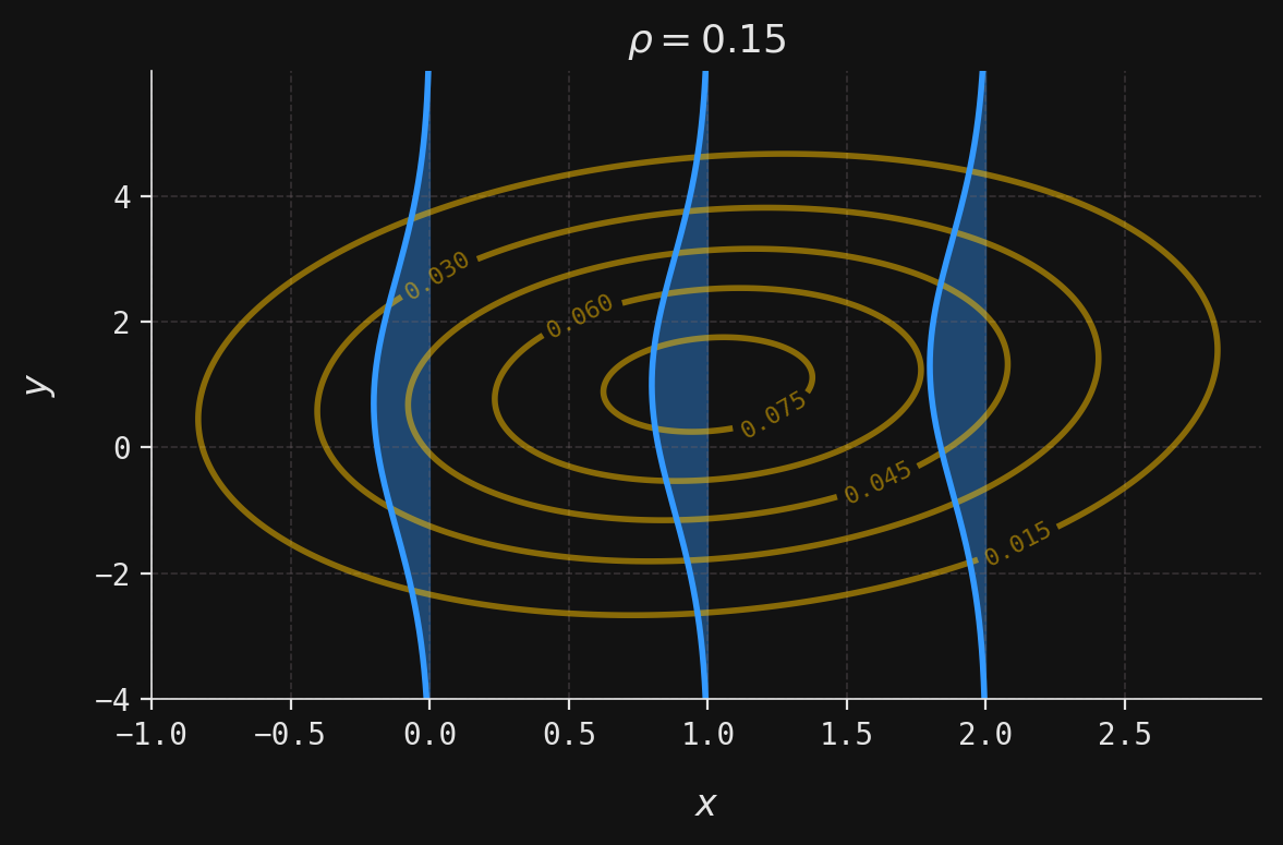
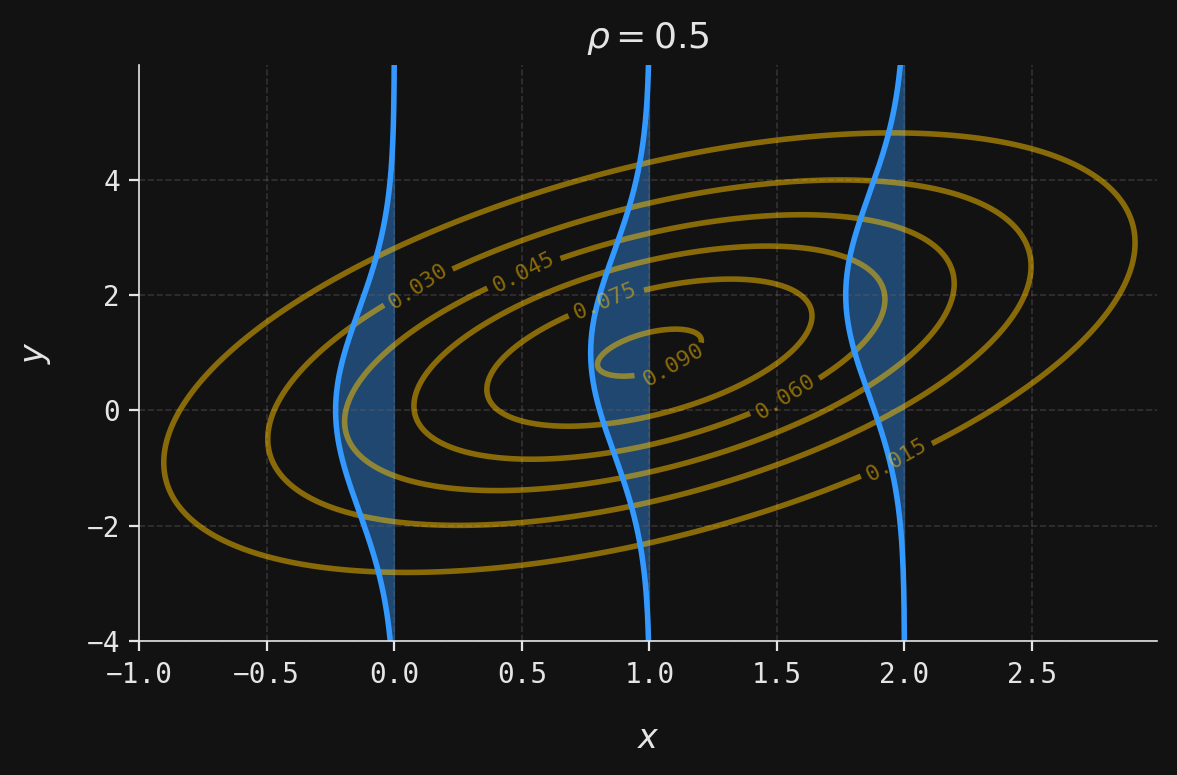
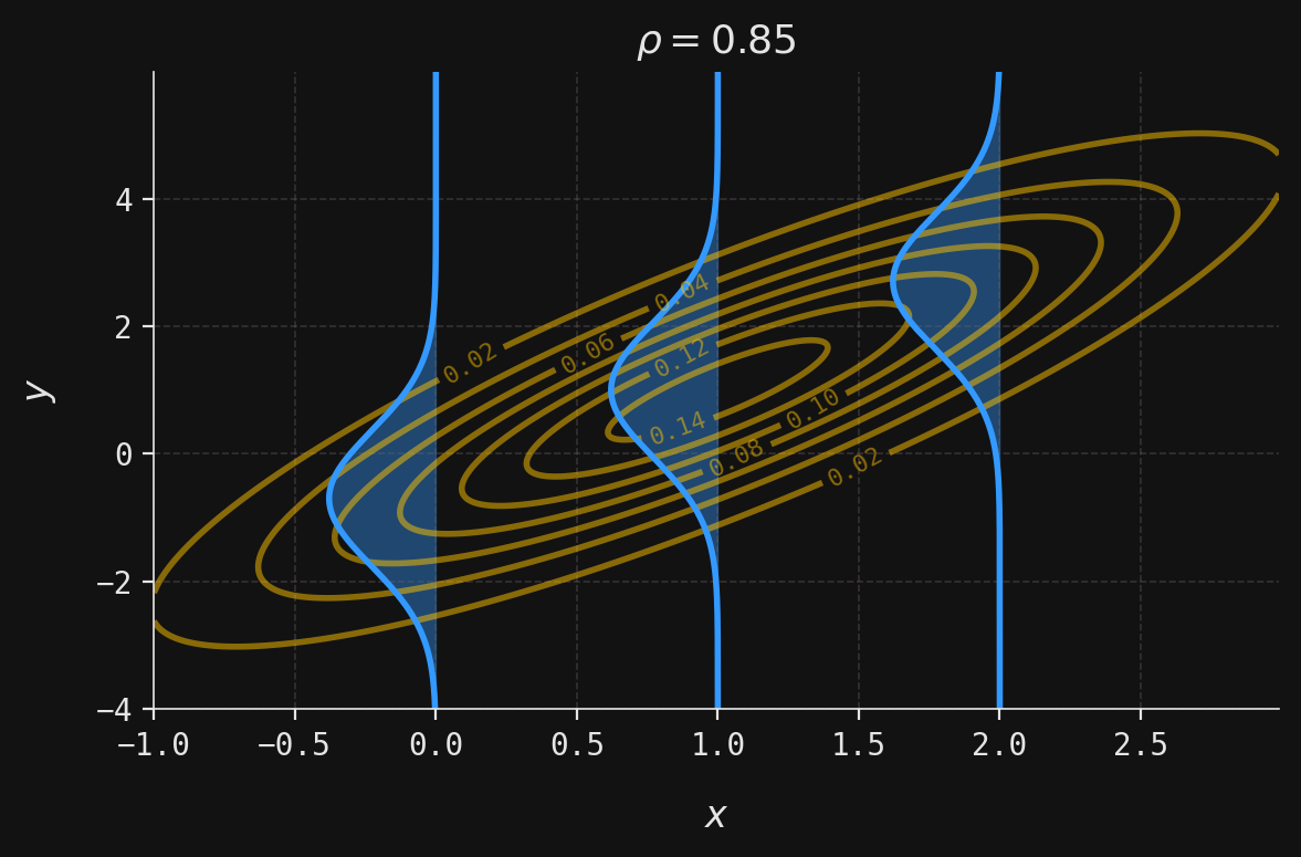
  ax.set_title(rf"$\rho ={rho}$")
  ax.set_xlabel(r"$x$")
  ax.set_ylabel(r"$y$")
  fig = plt.gcf()  # Get current figure
  fig.set_size_inches(6, 4)
  plt.tight_layout()
  plt.show()

_, ax = plt.subplots()
x, y = np.mgrid[-1:3:0.01, -4:6:0.01]

muX = 1
muY = 1
sigmaX = 1
sigmaY = 2
rho = 0.15

plot_combined(ax, muX, muY, sigmaX, sigmaY, rho, x, y, x_obs=[0, 1, 2], labels=True)

_, ax = plt.subplots()
rho = 0.5
plot_combined(ax, muX, muY, sigmaX, sigmaY, rho, x, y, x_obs=[0, 1, 2], labels=True)

_, ax = plt.subplots()
rho = 0.85
plot_combined(ax, muX, muY, sigmaX, sigmaY, rho, x, y, x_obs=[0, 1, 2], labels=True)

Conclusion