How do we mathematically represent what someone knows? This question sits at the heart of probability theory, information theory, and decision-making under uncertainty. When an experiment produces an outcome but we don’t observe it directly, our knowledge is partial: we might know some facts about the outcome while remaining uncertain about others. This partial knowledge needs a precise mathematical framework.
Consider a simple scenario: three coin flips produce a binary sequence like \(011\) or \(101\) where a \(0\) indicates that a tail was produced and \(1\) a head, but you don’t see the full result. If someone tells you only the outcome of the first flip, you’ve gained information, but how much? If they then reveal the second flip, you learn more, but again, how much? These questions about information content and uncertainty reduction require both a qualitative structure (what can you distinguish?) and a quantitative measure (how uncertain are you?).
The qualitative structure is captured by algebras of sets, which formalize the collection of events an observer can decide about. If you know the first flip, you can decide whether the full sequence starts with \(0\) or \(1\), partitioning the eight possible outcomes into two groups. Knowing the first two flips refines this partition into four groups, and so on. Each partition represents a distinct “information state,” and the nested structure
But algebras alone don’t quantify uncertainty; they only describe logical structure. To measure how much information each partition contains, we need entropy, along with the related notions of conditional entropy and mutual information. As partitions refine, conditional entropy decreases (less residual uncertainty) while mutual information increases (more shared information between algebras).
In a previous post, we introduced entropy, conditional entropy, and mutual information for probability distributions on finite sets. Here, we develop the same ideas from a measure-theoretic perspective, showing how information naturally emerges from the algebraic structure of events. This dual perspective (probabilistic and set-theoretic) provides both conceptual clarity and the foundation for extensions to infinite spaces, stochastic processes, and dynamical systems.
We’ll work primarily with a concrete example: three coin flips and the nested algebras they generate. Through explicit computations in R, we’ll see how entropy quantifies information at each stage of learning. The mathematical machinery we develop (algebras, partitions, and their correspondence) forms the backbone of modern probability theory. These ideas have powerful applications in gambling problems and games of chance, where players accumulate information over time, and in options pricing in mathematical finance, where nested filtrations model traders’ evolving information and determine fair prices for derivative securities. We will explore these latter themes in future posts.
The idea that algebras (and their \(\sigma\)-algebra generalizations) can represent “information states” is familiar to probability theorists. For example, these ideas appear throughout (Billingsley 1995), which also discusses gambling strategies, while (Björk 2020) provides a perspective from mathematical finance. Information-theoretic measures like entropy are applied to \(\sigma\)-algebras in ergodic theory and other areas; for an introduction, see (Walters 1982).
If you’d like to follow along with the code examples in this post, please see the dropdown code block below for the usual imports and setup.
Code
# Load required packageslibrary("ggplot2") # For plottinglibrary("knitr") # For table formatting (used with kable())library("dplyr") # For data manipulationlibrary("latex2exp") # For LaTeX rendering in plots# Source custom theme file# Note: Replace this path with your own theme file locationsource("../../aux-files/custom-theme.R")# Extract custom colors from theme# Note: These color definitions depend on your custom theme fileyellow <- custom_colors[["yellow"]]blue <- custom_colors[["blue"]]# Apply custom ggplot2 themetheme_set(custom_theme())
Algebras as information carriers
An observer monitors the result of some experiment. The set of all possible results is collected into a sample space\(\Omega\), whose elements \(\omega\) are called outcomes or sample points. Suppose that the experiment is finished, so that a definite \(\omega_0\) in \(\Omega\) is produced, but that the exact identity of \(\omega_0\) remains unknown to the observer. However, suppose that the observer has access to a set \(\mathcal{F}\) of subsets of \(\Omega\) with the following property:
For each \(A\in \mathcal{F}\), the observer can decide whether \(\omega_0\in A\) or not.
The observer’s decisions reflect the information they possess, so we can treat the class \(\mathcal{F}\) as a proxy for that information. Sets in \(\mathcal{F}\) are called (decidable) events. If the observer confirms that \(\omega_0\in A\) for some \(A\in \mathcal{F}\), then we say that “the event \(A\) has occurred”.
It is never in question that \(\omega_0\in \Omega\), since the same space \(\Omega\) contains all possible outcomes, so it is natural to include \(\Omega\) in the class \(\mathcal{F}\) of decidable events. But what other properties must \(\mathcal{F}\) have?
If the observer can determine whether an event \(A\) has occurred, then they obviously can determine whether \(A\) did not occur. This means that if \(A\in \mathcal{F}\), then \(A^c \in \mathcal{F}\) too.
If the observer can determine separately whether events \(A\) and \(B\) have occurred, then they can determine whether \(A\)or\(B\) has occurred. Since \(A\cup B\) consists of those outcomes that are either in \(A\) or \(B\), this means that \(A\cup B\) must be in \(\mathcal{F}\) when both \(A\) and \(B\) are.
Similarly, if the observer can determine separately whether events \(A\) and \(B\) have occurred, then they can determine whether \(A\)and\(B\) has occurred. This implies that \(\mathcal{F}\) must contain the intersection \(A\cap B\) whenever it contains both \(A\) and \(B\).
Here, \(A^c\) is the absolute complement of \(A\), consisting of those \(\omega\in \Omega\) that are not in \(A\).
These three properties capture what it means for the observer’s collection of events \(\mathcal{F}\) to represent a logically coherent state of information. They lead us naturally to the formal definition of an algebra of sets.
Actually, we need not explicitly require that \(\mathcal{F}\) contains all (binary) intersections of events, since this follows from properties (1) and (2). Note also that \(\mathcal{F}\) must contain the empty set, since it contains \(\Omega\) and is closed under complements.
Definition 1 Let \(\mathcal{F}\) be a set of subsets of a set \(\Omega\). Then \(\mathcal{F}\) is called an algebra of sets (in \(\Omega\)) if it has the following properties:
We have thus argued that our class \(\mathcal{F}\) of decidable events—encoding our observer’s information—must be an algebra of sets in the sample space \(\Omega\).
As we indicated in the margin note above, algebras of sets are also closed under binary intersections. Moreover, an easy inductive proof shows that algebras are also closed under all finite unions and intersections, not just binary ones. In this post we’ll stick to finite sample spaces, but in the infinite case one usually strengthens these closure properties to include countable unions, yielding \(\sigma\)-algebras of sets.
Example: coin tosses
In practice, the information encoded in \(\mathcal{F}\) is often most naturally described by a partition that generates it. A partition is a collection of sets
\[
\{A_1,A_2,\ldots,A_n\}
\]
where each \(A_k \subset \Omega\), the sets \(A_k\) are mutually disjoint, and their union exhausts the sample space: \(\Omega = \bigcup_{k=1}^n A_k\).
The intuition is simple: an observer’s information typically comes from knowing the answer to some question. Each possible answer groups together certain outcomes, and these groups form a partition of \(\Omega\). The algebra \(\mathcal{F}\) is then the smallest algebra containing all sets in this partition. We will study partitions in more detail in the next section, but for now we see how it works in a simple example.
We consider the sample space \(\Omega\) consisting of all binary sequences of length 3:
We imagine that a binary sequence \(\omega\) in \(\Omega\) represents the result of flipping a coin three times in succession, with \(0\) when a tail occurs, and \(1\) when a head is shown. We let \(X_i(\omega)\) denote the result of the \(i\)-th flip in \(\omega\) (so \(X_i(\omega)=0\) or \(1\)), and we write
\[
Y = X_1 + X_2 + X_3.
\]
The four functions \(X_1\), \(X_2\), \(X_3\), and \(Y\) are, of course, random variables on \(\Omega\). If the coin has probability \(\theta\) of showing heads, then \(X_i \sim \mathcal{B}er(\theta)\) for each \(i\), and \(Y\sim \mathcal{B}in(3,\theta)\).
We will be carrying out some basic computations later, so let’s implement our scenario in the machine, by coding a data frame in which each row represents an outcome \(\omega\):
Code
# Create the sample space Omega as a data frame# Each row represents one of the 8 possible outcomes (binary sequences of length 3)Omega <-data.frame(X1 =c(0, 0, 0, 0, 1, 1, 1, 1), # First coin flip: 0 = tail, 1 = headX2 =c(0, 0, 1, 1, 0, 0, 1, 1), # Second coin flipX3 =c(0, 1, 0, 1, 0, 1, 0, 1) # Third coin flip)# Add random variable Y: total number of heads across all three flipsOmega <- Omega %>%mutate(Y = X1 + X2 + X3)# Display the sample space as a formatted tablekable( Omega,caption ="sample space $\\Omega$ and random variables $X_1$, $X_2$, $X_3$, and $Y$")
sample space \(\Omega\) and random variables \(X_1\), \(X_2\), \(X_3\), and \(Y\)
X1
X2
X3
Y
0
0
0
0
0
0
1
1
0
1
0
1
0
1
1
2
1
0
0
1
1
0
1
2
1
1
0
2
1
1
1
3
Now, suppose that the coin was flipped three times, producing a definite outcome \(\omega_0\) in \(\Omega\), but that its exact identity is unknown to our observer. The only information available is the answer to the question: “What is the outcome of the first flip?”. This information allows the observer to partition the sample space \(\Omega\) and generate an algebra \(\mathcal{F}_1\), just as we described at the beginning of this section.
is an algebra of sets in \(\Omega\). We would visualize this partition as follows:
Let’s insert a column in our data frame tracking the membership of each outcome \(\omega\) (i.e., row) in \(A_1\) or \(A_2\):
Code
# Group outcomes by the result of the first flip (X1)# and assign a group ID to track which partition set (A1 or A2) each outcome belongs toOmega <- Omega %>%group_by(X1) %>%mutate(Ai =cur_group_id()) %>%# Ai = 1 for A1 (X1=0), Ai = 2 for A2 (X1=1)ungroup() %>%as.data.frame()# Display the updated sample space showing partition membershipkable(Omega, caption ="column Ai records the index $i$ of $A_i$")
column Ai records the index \(i\) of \(A_i\)
X1
X2
X3
Y
Ai
0
0
0
0
1
0
0
1
1
1
0
1
0
1
1
0
1
1
2
1
1
0
0
1
2
1
0
1
2
2
1
1
0
2
2
1
1
1
3
2
Now, suppose the observer is also given the answer to the question: “What is the outcome of the second flip?” Combining this with the information from the first flip, the observer can now distinguish outcomes based on the results of the first two flips. This additional information generates a finer partition of \(\Omega\) and produces a second algebra \(\mathcal{F}_2\), which contains the first:
\[
\mathcal{F}_1 \subset \mathcal{F}_2.
\]
Inclusions of algebras represent refinements of information.
where \(B_1\) corresponds to the answer “first and second flips are both tails”, \(B_2\) to “first flip tail, second flip head”, and so on. The algebra that is generated by this partition is
As expected, \(\mathcal{F}_2\) contains \(\mathcal{F}_1\) since \(B_1\cup B_2 = A_1\) and \(B_3\cup B_4 = A_2\), reflecting that the observer’s information has been refined. Along with the first partition induced by \(\mathcal{F}_1\), we would visualize this finer partition as follows:
Let’s insert our new algebra into the machine:
Code
# Group outcomes by the results of the first two flips (X1 and X2)# and assign a group ID to track which partition set (B1, B2, B3, or B4) each outcome belongs toOmega <- Omega %>%group_by(X1, X2) %>%mutate(Bi =cur_group_id()) %>%# Bi = 1 for B1, Bi = 2 for B2, etc.ungroup() %>%as.data.frame()# Display the updated sample space showing partition membership for the refined algebra F2kable(Omega, caption ="column Bi records the index $i$ of $B_i$")
column Bi records the index \(i\) of \(B_i\)
X1
X2
X3
Y
Ai
Bi
0
0
0
0
1
1
0
0
1
1
1
1
0
1
0
1
1
2
0
1
1
2
1
2
1
0
0
1
2
3
1
0
1
2
2
3
1
1
0
2
2
4
1
1
1
3
2
4
Finally, suppose the observer is given the answer to the question: “What is the outcome of the third flip?” With this information, the observer can now distinguish outcomes based on all three flips, completely specifying \(\omega_0\). This generates the finest partition of \(\Omega\) and produces a third algebra \(\mathcal{F}_3\), which refines the information in \(\mathcal{F}_2\) (and thus also \(\mathcal{F}_1\)):
where each \(C_i\) corresponds to the answer to the question, “Which sequence of heads and tails occurred in all three flips?”. Knowing which singleton contains \(\omega_0\) completely identifies the outcome. To form an algebra, \(\mathcal{F}_3\) must include not only these singletons but also all possible unions of them; in other words, \(\mathcal{F}_3\) is the power set of \(\Omega\), containing all subsets of the sample space. Along with the first two partitions induced by \(\mathcal{F}_1\) and \(\mathcal{F}_2\), we would visualize this finest partition as follows:
We insert one last column in our data frame for the \(C_i\)’s:
Code
# Group outcomes by all three flips (X1, X2, and X3)# Each combination of (X1, X2, X3) uniquely identifies one outcomeOmega <- Omega %>%group_by(X1, X2, X3) %>%mutate(Ci =cur_group_id()) %>%# Ci = 1 for C1, Ci = 2 for C2, etc.ungroup() %>%as.data.frame()# Display the updated sample space showing the finest partition (singletons)# At this level, each outcome is completely distinguishablekable(Omega, caption ="column Ci records the index $i$ of $C_i$")
column Ci records the index \(i\) of \(C_i\)
X1
X2
X3
Y
Ai
Bi
Ci
0
0
0
0
1
1
1
0
0
1
1
1
1
2
0
1
0
1
1
2
3
0
1
1
2
1
2
4
1
0
0
1
2
3
5
1
0
1
2
2
3
6
1
1
0
2
2
4
7
1
1
1
3
2
4
8
To recap, the sets \(A_k\), \(B_k\), and \(C_k\) form partitions of \(\Omega\), with each successive partition being finer than the last: each \(A_k\) is a union of \(B_k\)’s, and each \(B_k\) is a union of \(C_k\)’s. These sets are also the atoms of their respective algebras, meaning they do not properly contain any nonempty subset in the corresponding algebra.
Two outcomes \(\omega_1\) and \(\omega_2\) in the same \(A_k\) are indistinguishable using only the information in \(\mathcal{F}_1\). Likewise, outcomes in the same \(B_k\) are indistinguishable with respect to \(\mathcal{F}_2\). The \(C_k\), by contrast, correspond to complete information in \(\mathcal{F}_3\), so no ambiguity remains.
captures a distinct level of information about the outcome \(\omega_0\). This nested structure provides a simple model of learning over time: as the experiment unfolds and the observer acquires new data, their algebra of decidable events expands, splitting sets of previously indistinguishable outcomes into finer partitions—until, at last, \(\mathcal{F}_3\) represents complete knowledge of \(\omega_0\).
Algebras and partitions
In this section, we nail down the ideas from the previous section on partitions and algebras and highlight four useful theorems connecting them. Some proofs get a bit technical, so feel free to skim and focus on the statements. For simplicity, we stick to finite sets \(\Omega\), though many results hold for infinite sets too.
So, let \(\Omega\) be a finite set and \(\mathcal{F}\) an algebra of sets in \(\Omega\). Indistinguishability of two elements \(\omega\) and \(\omega'\) of \(\Omega\) (relative to \(\mathcal{F}\)) occurs exactly when we have
\[
\omega \in A \quad \Leftrightarrow \quad \omega' \in A, \quad \forall A\in \mathcal{F}.
\tag{2}\]
Elements \(\omega\) and \(\omega'\) related in this way will be called \(\mathcal{F}\)-equivalent.
This notion of equivalence is evidently an equivalence relation in the technical sense, and thus we obtain a partition of \(\Omega\) into the distinct equivalence classes. These equivalence classes are actually themselves contained in \(\mathcal{F}\), since \(\mathcal{F}\) is closed under intersections. In fact, if \(E\) is an equivalence class containing an outcome \(\omega\in \Omega\), then \(E\) is the intersection of all \(A\in \mathcal{F}\) that contain \(\omega\):
\[
E = \bigcap_{\omega \in A \in \mathcal{F}} A.
\]
(Verification of this equality is left to the reader.) But even more than being elements of \(\mathcal{F}\), these equivalence classes are atomic in the sense of the following definition.
Definition 2 Let \(\mathcal{F}\) be an algebra of sets in a finite set \(\Omega\). A set \(A\in \mathcal{F}\) is called an atom if it is non-reducible, in the sense that \(A\) contains no nonempty subset of \(\mathcal{F}\) other than itself.
Theorem 1 (Atomic theorm) Let \(\mathcal{F}\) be an algebra of sets in a finite set \(\Omega\).
There exists a partition \(\mathcal{A}\) of \(\Omega\) consisting entirely of atoms in \(\mathcal{F}\). In fact, \(\mathcal{A}\) may be chosen to consist of the distinct \(\mathcal{F}\)-equivalence classes.
If \(\mathcal{A}\) is a partition of \(\Omega\) consisting of atoms in \(\mathcal{F}\), then every nonempty set in \(\mathcal{F}\) is a union of atoms in \(\mathcal{A}\).
Let \(\mathcal{A}\) and \(\mathcal{B}\) be two partitions of \(\Omega\) consisting of atoms in \(\mathcal{F}\). Then \(\mathcal{A}= \mathcal{B}\).
NoteProof.
(1): Since the distinct \(\mathcal{F}\)-equivalence classes partition \(\Omega\), we just need to show that a given equivalence class is non-reducible. So, let \(E\) be an \(\mathcal{F}\)-equivalence class, and suppose that \(A\in \mathcal{F}\) is a nonempty subset of \(E\). Choose \(\omega'\in A\) and \(\omega \in E\). Then \(\omega'\in E\) as well, and so \(\omega\) and \(\omega'\) are \(\mathcal{F}\)-equivalent. But then \(\omega'\in A\) implies \(\omega\in A\), and since \(\omega\) was an arbitrarily chosen element of \(E\), we must have \(E\subset A\). But \(A\) began as a subset of \(E\), and so \(E=A\).
(2): Since the atoms in \(\mathcal{A}\) partition \(\Omega\), it will suffice to show that every nonempty set \(S\in \mathcal{F}\) is either disjoint from a given atom in \(A\in\mathcal{A}\), or \(S\) contains \(A\) as a subset. But if \(S\cap A\) is nonempty, then we must have \(S\cap A = A\) since \(S\cap A\in \mathcal{F}\) and \(A\) is non-reducible. But then \(A\subset S\), as desired.
(3): First, choose an atom \(A\in \mathcal{A}\). Since \(\mathcal{B}\) is a partition of \(\Omega\), there must exist a \(B\in \mathcal{B}\) such that \(A\cap B\) is nonempty. But then
\[
A = A\cap B =B,
\]
where the first equalities follow from the fact that \(A\cap B\) is in \(\mathcal{F}\) and non-reducibility of \(A\) and \(B\). Thus \(A\in \mathcal{B}\), which proves \(\mathcal{A}\subset \mathcal{B}\). A symmetric argument proves the opposite containment, and hence \(\mathcal{A}= \mathcal{B}\).
So, every algebra of sets \(\mathcal{F}\) in a finite set \(\Omega\) naturally gives rise to a unique partition \(\mathcal{A}\) of \(\Omega\) consisting of atoms in \(\mathcal{F}\). Conversely, as we saw in the coin-flip example, a given partition \(\mathcal{A}\) of \(\Omega\) can be used to generate an algebra, which we denote by \(\sigma(\mathcal{A})\). By construction, \(\sigma(\mathcal{A})\) is the smallest algebra in \(\Omega\) that contains all sets in \(\mathcal{A}\), i.e., \(\mathcal{A}\subset \sigma(\mathcal{A})\).
Theorem 2 (Generating algebras via atoms) Let \(\mathcal{A}\) be a partition of a finite set \(\Omega\).
Every set in \(\sigma(\mathcal{A})\) is a union of sets in \(\mathcal{A}\).
The sets in \(\mathcal{A}\) are atoms in the algebra \(\sigma(\mathcal{A})\).
To see this theorem in action, I encourage you to scroll back and look at the algebra \(\mathcal{F}_2\) in (1) in the previous section, generated by the partition \(\{B_1,B_2,B_3,B_4\}\). Notice that \(\mathcal{F}_2\) does indeed consist of all unions of the \(B_k\)’s.
NoteProof.
(1): Since \(\sigma(\mathcal{A})\) is an algebra, it must contain the set \(\mathcal{F}\) of all unions of sets in \(\mathcal{A}\), so we have
The point is that \(\mathcal{F}\) is already an algebra, and hence \(\mathcal{F}= \sigma(\mathcal{A})\). To prove this, note that \(\Omega \in \mathcal{F}\) since the union of all sets in \(\mathcal{A}\) is \(\Omega\). Clearly \(\mathcal{F}\) is closed under unions, so we need only show that it is closed under absolute complements. But because the sets in \(\mathcal{A}\) are pairwise disjoint and their union is \(\Omega\), the complement of a union of sets in \(\mathcal{A}\) is another set of the same form, and hence \(\mathcal{F}\) is indeed closed under unions. This proves the claim \(\mathcal{F}= \sigma(\mathcal{A})\), and thereby establishes the first statement.
(2): Let \(A\in \mathcal{A}\) and suppose \(S\in \mathcal{F}\) is a nonempty subset of \(A\). But then \(S\) is a union of sets in \(\mathcal{A}\), and since the sets in \(\mathcal{A}\) are pairwise disjoint, we must have \(S=A\).
The mapping \(\mathcal{A}\mapsto \sigma(\mathcal{A})\) associating every partition \(\mathcal{A}\) of a finite set \(\Omega\) with the algebra \(\sigma(\mathcal{A})\) is injective. Indeed, if \(\mathcal{A}\) and \(\mathcal{B}\) are two partitions such that \(\sigma(\mathcal{A}) = \sigma(\mathcal{B})\), then Theorem 2 shows that \(\mathcal{A}\) and \(\mathcal{B}\) are both partitions of the same algebra and both consist of atoms; then Theorem 1 shows \(\mathcal{A}= \mathcal{B}\). On the other hand, if \(\mathcal{F}\) is an algebra of sets in \(\Omega\), then a partition \(\mathcal{A}\) of \(\Omega\) consisting of atoms in \(\mathcal{F}\) exists, by Theorem 1, and all sets in \(\mathcal{F}\) are unions of atoms. But then \(\mathcal{F}= \sigma(\mathcal{A})\) by Theorem 2. We have thus proved:
Theorem 3 (Algebras \(=\) Partitions) Let \(\Omega\) be a finite set. The mapping \(\mathcal{A}\mapsto \sigma(\mathcal{A})\) is a bijection from the class of all partitions of \(\Omega\) onto the class of all algebras of sets in \(\Omega\).
Finally, if \(\mathcal{F}\) and \(\mathcal{G}\) are two algebras of sets in \(\Omega\), we say \(\mathcal{F}\)refines\(\mathcal{G}\) if \(\mathcal{G}\subset \mathcal{F}\). As we saw in the coin-flip example, refinements of algebras corresponds to refinement of information.
Theorem 4 (Refinement Theorem) Let \(\mathcal{F}\) and \(\mathcal{G}\) be two algebras of sets in a finite set \(\Omega\) with associated partitions \(\mathcal{A}\) and \(\mathcal{B}\) consisting of atoms, respectively. Then \(\mathcal{F}\) refines \(\mathcal{G}\) if and only if every set \(B\in \mathcal{B}\) is a union of sets in \(\mathcal{A}\).
NoteProof.
First, supposing that \(\mathcal{F}\) refines \(\mathcal{G}\), we have
where the two equalities follow from Theorem 3. The desired conclusion then follows from part (1) of Theorem 2. Conversely, if every \(B\in \mathcal{B}\) is a union of sets in \(\mathcal{A}\), then we get the subset containment in
where the equality follows (one more time) from Theorem 3 and the subset containment from the fact \(\mathcal{F}\) is an algebra containing \(\mathcal{B}\). Thus \(\mathcal{F}\) refines \(\mathcal{G}\).
The correspondence between algebras and partitions gives us two complementary perspectives on information. The algebraic view emphasizes logical operations: we can decide membership in events, take complements, form unions and intersections. The partition view emphasizes distinguishability: outcomes in the same partition set are indistinguishable, while outcomes in different sets can be told apart. Theorem 3 shows these perspectives are equivalent—every algebra uniquely determines a partition of atoms, and every partition uniquely generates an algebra. Moreover, Theorem 4 shows that refinement of information has a natural interpretation in both frameworks: \(\mathcal{F}\) refines \(\mathcal{G}\) (as algebras) precisely when the atoms of \(\mathcal{F}\) subdivide the atoms of \(\mathcal{G}\) (as partitions). This duality between set-theoretic structure and equivalence classes will prove essential when we introduce entropy, where the partition view naturally connects to probability distributions over distinguishable outcomes.
Algebras and entropy
Having established the correspondence between algebras and partitions, we now turn to quantifying the information content they represent. While the nested structure
that we explored in our coin-flip example shows that information is refined—that uncertainty decreases—we have not yet measured how much uncertainty remains at each stage, or how much uncertainty is removed by each refinement. To do this, we introduce the concept of entropy associated with an algebra of sets, which is a natural extension of the Shannon entropy of a random variable that we studied in a previous post.
We continue to work with a finite sample space \(\Omega\) and an algebra \(\mathcal{F}\) of sets in \(\Omega\). To quantify uncertainty, we need a probability measure \(P\) on \(\Omega\), which assigns a probability \(P(\{\omega\})\) to each outcome \(\omega\in \Omega\). The probability of an event \(A\in \mathcal{F}\) is then given by
\[
P(A) = \sum_{\omega \in A} P(\{\omega\}).
\]
Together, the triple \((\Omega,\mathcal{F},P)\) is called a finite probability space. An algebra of sets \(\mathcal{G}\) in \(\Omega\) is called a sub-\(\sigma\)-algebra of \(\mathcal{F}\) if \(\mathcal{G}\subset \mathcal{F}\).
In our coin-flip example, we can define a probability measure \(P\) on \(\Omega\) by assuming that the coin has probability \(\theta\) of showing heads on any given flip, independently of previous flips. Then the probability of an outcome \(\omega\) with \(Y(\omega)\) heads is
If we suppose that \(\theta = 0.6\), then the probabilties on \(\Omega\) are as follows:
Code
theta <-0.6# Probability of heads (coin bias parameter)# Calculate the probabilities of each outcome in Omega# Under independence, P({ω}) = θ^(# heads) × (1-θ)^(# tails)Omega <- Omega %>%mutate(p = (theta^Y) * ((1- theta)^(3- Y)) # Probability based on binomial model )# Display the sample space with probabilities as a formatted table# Each row shows an outcome ω and its probability P({ω})kable( Omega,caption ="sample space $\\Omega$ with probabilities $P(\\{\\omega\\})$ for each outcome $\\omega$")
sample space \(\Omega\) with probabilities \(P(\{\omega\})\) for each outcome \(\omega\)
X1
X2
X3
Y
Ai
Bi
Ci
p
0
0
0
0
1
1
1
0.064
0
0
1
1
1
1
2
0.096
0
1
0
1
1
2
3
0.096
0
1
1
2
1
2
4
0.144
1
0
0
1
2
3
5
0.096
1
0
1
2
2
3
6
0.144
1
1
0
2
2
4
7
0.144
1
1
1
3
2
4
8
0.216
With finite probability spaces defined, we can now introduce the entropy of an algebra of sets, which measures the uncertainty associated with the information it encodes. The definition is a straightforward extension of Shannon entropy, applied to the partition of \(\Omega\) formed by the atoms of the algebra.
Definition 3 Let \((\Omega,\mathcal{F},P)\) be a finite probability space, let \(\mathcal{G}\) be a sub-\(\sigma\)-algebra of \(\mathcal{F}\), and let \(\{B_1,B_2,\ldots,B_n\}\) be the partition of \(\Omega\) by atoms of \(\mathcal{G}\). We then define the entropy of \(\mathcal{G}\) to be the quantity
For those readers who are familiar with abstract integration theory, we note that the formula (3) can be expressed as a Lebesgue integral. Indeed, if we write \(\pi: \Omega \to \Omega/\mathcal{G}\) for the natural projection map onto the quotient space \(\Omega/\mathcal{G}\) whose points are the atoms of \(\mathcal{G}\), then the entropy of \(\mathcal{G}\) is given by the Lebesgue integral
where \(s:\Omega/\mathcal{G}\to \mathbb{R}\) is the surprisal function given by
\[
s(B) = -\log{P(B)},
\]
and \(\pi_\ast P\) is the pushforward measure of \(P\) under \(\pi\) defined on the power set of the quotient \(\Omega/\mathcal{G}\). By the substitution rule, we also have
so the entropy is nothing but the expected value \(E(s\circ \pi)\) of the random variable \(s\circ \pi\) on \(\Omega\). This abstraction becomes essential for infinite sample spaces, but we won’t need it here.
Returning to our coin-flip example, we can now compute the entropies of the three algebras \(\mathcal{F}_1\), \(\mathcal{F}_2\), and \(\mathcal{F}_3\) that we constructed. First, we summarize the probabilities of the atoms in each algebra:
Code
# Calculate probabilities on the atoms of F1# For algebra F1 with partition {A1, A2}, sum the probabilities of outcomes in each atomF1_probs <- Omega %>%group_by(Ai) %>%# Group by atom membership (Ai = 1 or 2)summarise(p =sum(p)) # Sum probabilities of all outcomes in each atom# Display the probabilities for atoms of F1 as a formatted tablekable( F1_probs,caption ="probabilities $P(A_i)$ for the atoms $A_i$ of algebra $\\mathcal{F}_1$")
probabilities \(P(A_i)\) for the atoms \(A_i\) of algebra \(\mathcal{F}_1\)
Ai
p
1
0.4
2
0.6
Code
# Calculate probabilities on the atoms of F2# For algebra F2 with partition {B1, B2, B3, B4}, sum probabilities for each atomF2_probs <- Omega %>%group_by(Bi) %>%# Group by atom membership (Bi = 1, 2, 3, or 4)summarise(p =sum(p)) # Sum probabilities of all outcomes in each atom# Display the probabilities for atoms of F2 as a formatted tablekable( F2_probs,caption ="probabilities $P(B_i)$ for the atoms $B_i$ of algebra $\\mathcal{F}_2$")
probabilities \(P(B_i)\) for the atoms \(B_i\) of algebra \(\mathcal{F}_2\)
Bi
p
1
0.16
2
0.24
3
0.24
4
0.36
Code
# Calculate probabilities on the atoms of F3# For algebra F3 with partition {C1, ..., C8} (singletons), extract individual outcome probabilitiesF3_probs <- Omega %>%group_by(Ci) %>%# Group by atom membership (Ci = 1 through 8)summarise(p =sum(p)) # Sum probabilities (each atom contains exactly one outcome)# Display the probabilities for atoms of F3 as a formatted table# Since F3 is the power set, each atom Ci corresponds to a single outcome ωkable( F3_probs,caption ="probabilities $P(C_i)$ for the atoms $C_i$ of algebra $\\mathcal{F}_3$")
probabilities \(P(C_i)\) for the atoms \(C_i\) of algebra \(\mathcal{F}_3\)
Ci
p
1
0.064
2
0.096
3
0.096
4
0.144
5
0.096
6
0.144
7
0.144
8
0.216
Since the algebra \(\mathcal{F}_3\) is the power set on \(\Omega\), notice that the probabilties of the atoms in \(\mathcal{F}_3\) are just the probabilities of the individual outcomes in \(\Omega\).
We now compute the entropies of the three algebras:
Code
# Calculate entropy using H = -sum(p * log(p))# This formula computes Shannon entropy, measuring uncertainty in the distribution# Calculate marginal entropy H(F1)# For algebra F1 with atoms {A1, A2}, compute entropy over the 2-element partitionH_F1 <- F1_probs %>%mutate(surprisal =-log(p)) %>%# Surprisal: -log(p) for each atom's probabilitysummarise(H =sum(p * surprisal)) %>%# Entropy: expected surprisalpull(H) # Extract the scalar value# Calculate marginal entropy H(F2)# For algebra F2 with atoms {B1, B2, B3, B4}, compute entropy over the 4-element partitionH_F2 <- F2_probs %>%mutate(surprisal =-log(p)) %>%summarise(H =sum(p * surprisal)) %>%pull(H)# Calculate marginal entropy H(F3)# For algebra F3 with atoms {C1, ..., C8}, compute entropy over the 8-element partition# F3 corresponds to complete information (the power set of Omega)H_F3 <- F3_probs %>%mutate(surprisal =-log(p)) %>%summarise(H =sum(p * surprisal)) %>%pull(H)# Create a tibble containing the three entropy values# Shows how entropy increases as algebras refine: H(F1) < H(F2) < H(F3)marginal_entropies <-tibble(entropy =c("H(F1)", "H(F2)", "H(F3)"), # Labels for each algebravalue =c(H_F1, H_F2, H_F3) # Corresponding entropy values in nats)# Display the marginal entropies as a formatted tablekable( marginal_entropies,caption ="marginal entropies for algebras $\\mathcal{F}_1$, $\\mathcal{F}_2$, and $\\mathcal{F}_3$")
marginal entropies for algebras \(\mathcal{F}_1\), \(\mathcal{F}_2\), and \(\mathcal{F}_3\)
entropy
value
H(F1)
0.6730117
H(F2)
1.3460233
H(F3)
2.0190350
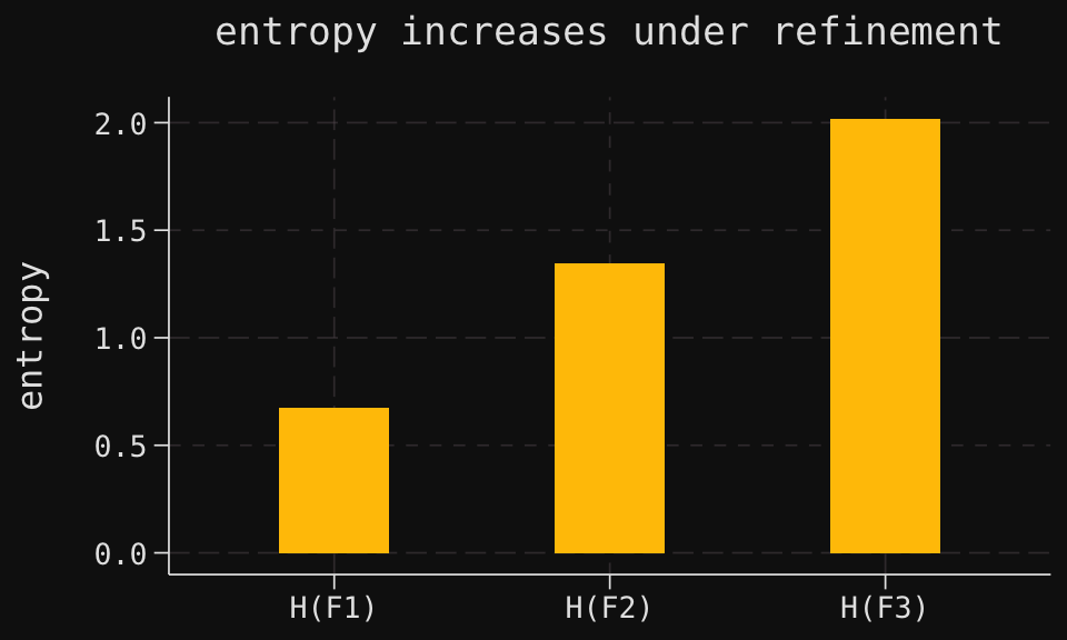
Thus, we see that the entropy increases as we refine our information. This means that uncertainty increases as our information becomes more detailed, which may seem counterintuitive at first glance. However, this is a natural consequence of the way entropy is defined: it measures the expected uncertainty over all possible outcomes, and as we refine our information, we are effectively considering a larger number of possible outcomes (the atoms of the finer algebra), each with its own associated probability. The increased granularity leads to a higher overall uncertainty when averaged across all outcomes.
We may visualize this increase in entropy as follows, where reading the plot from left to right corresponds to refining our information from \(\mathcal{F}_1\) to \(\mathcal{F}_2\) to \(\mathcal{F}_3\):
Code
# Create a bar chart visualizing how entropy increases across the filtration# Each bar represents the entropy H(Fi) for i = 1, 2, 3ggplot(marginal_entropies, aes(x = entropy, y = value)) +geom_col(fill = yellow, width =0.4) +# Yellow bars with reduced width for claritylabs(title ="entropy increases under refinement", # Title describes the key patternx =NULL, # Remove x-axis label (entropy names are self-explanatory)y ="entropy"# Label y-axis with the quantity being measured )
Having defined the entropy of an algebra, we can now introduce two related concepts: conditional entropy and mutual information. These quantities measure, respectively, the uncertainty remaining in one algebra given knowledge of another, and the amount of information shared between two algebras.
To define the conditional entropy, we need two sub-\(\sigma\)-algebras \(\mathcal{G}\) and \(\mathcal{H}\) of a finite probability space \((\Omega,\mathcal{F},P)\). If the decompositions of \(\Omega\) into the atoms of \(\mathcal{G}\) and \(\mathcal{H}\) are
respectively, then the decomposition of \(\Omega\) into the atoms of the algebra \(\mathcal{G}\vee \mathcal{H}\), the smallest algebra containing both \(\mathcal{G}\) and \(\mathcal{H}\), is given by the nonempty sets among \(B_i \cap C_j\) for each of \(i=1,2,\ldots,n\) and \(j=1,2,\ldots,m\).
Definition 4 Let \((\Omega,\mathcal{F},P)\) be a finite probability space, and let \(\mathcal{G}\) and \(\mathcal{H}\) be two sub-\(\sigma\)-algebras of \(\mathcal{F}\). The conditional entropy of \(\mathcal{G}\) given \(\mathcal{H}\) is the quantity
The intuition for this definition is as follows. The entropy \(H(\mathcal{H})\) measures the uncertainty in \(\mathcal{H}\), while \(H(\mathcal{G}\vee \mathcal{H})\) measures the uncertainty in the combined information of \(\mathcal{G}\) and \(\mathcal{H}\). The difference between these two quantities, \(H(\mathcal{G}\mid \mathcal{H})\), thus represents the uncertainty that remains in \(\mathcal{G}\) once we know everything in \(\mathcal{H}\).
In our coin-flip example, three conditional entropies are of interest: \(H(\mathcal{F}_3\mid \mathcal{F}_i)\), for each of \(i=1,2,3\). Since we have the nested sequence
and similarly for \(H(\mathcal{F}_3 \mid \mathcal{F}_2)\) and \(H(\mathcal{F}_3 \mid \mathcal{F}_3)\). In particular, we have that \(H(\mathcal{F}_3 \mid \mathcal{F}_3) =0\), which squares with our intuition that, given the information in \(\mathcal{F}_3\), the uncertainty remaining in \(\mathcal{F}_3\) is zero.
We compute all three conditional entropies:
Code
# Create a tibble containing conditional entropy values for the filtration# For nested algebras F1 ⊂ F2 ⊂ F3, conditional entropy H(F3 | Fi) = H(F3) - H(Fi)# This measures the residual uncertainty in F3 given knowledge of Ficonditional_entropies <-tibble(entropy =c("H(F3 | F1)", "H(F3 | F2)", "H(F3 | F3)"), # Labels for each conditional entropyvalue =c(H_F3 - H_F1, H_F3 - H_F2, H_F3 - H_F3) # Values: H(F3 | Fi) for each i)# Display the conditional entropies as a formatted table# Shows how residual uncertainty in F3 decreases as we refine from F1 to F2 to F3kable( conditional_entropies,caption ="conditional entropies for the filtration $\\mathcal{F}_1 \\subset \\mathcal{F}_2 \\subset \\mathcal{F}_3$")
conditional entropies for the filtration \(\mathcal{F}_1 \subset \mathcal{F}_2 \subset \mathcal{F}_3\)
entropy
value
H(F3 | F1)
1.3460233
H(F3 | F2)
0.6730117
H(F3 | F3)
0.0000000
These values show that as we compute \(H(\mathcal{F}_3 \mid \mathcal{F}_i)\) along the sequence
the conditional entropies decrease. This reflects the fact that as we refine our information (moving from \(\mathcal{F}_1\) to \(\mathcal{F}_2\) to \(\mathcal{F}_3\)), the uncertainty remaining in \(\mathcal{F}_3\) given knowledge of the other algebras diminishes. This aligns perfectly with our intuition: more information leads to less uncertainty.
Finally, we define the mutual information between two sub-\(\sigma\)-algebras \(\mathcal{G}\) and \(\mathcal{H}\) of a finite probability space \((\Omega,\mathcal{F},P)\). This quantity measures the amount of information shared between \(\mathcal{G}\) and \(\mathcal{H}\), quantifying how much knowing one reduces uncertainty about the other.
Definition 5 Let \((\Omega,\mathcal{F},P)\) be a finite probability space, and let \(\mathcal{G}\) and \(\mathcal{H}\) be two sub-\(\sigma\)-algebras of \(\mathcal{F}\). The mutual information between \(\mathcal{G}\) and \(\mathcal{H}\) is the quantity
The intuition for this definition is as follows. The entropy \(H(\mathcal{G})\) measures the uncertainty in \(\mathcal{G}\). The conditional entropy \(H(\mathcal{G}\mid \mathcal{H})\) measures the uncertainty remaining in \(\mathcal{G}\) once we know everything in \(\mathcal{H}\). The difference between these two quantities, \(I(\mathcal{G},\mathcal{H})\), thus represents the reduction in uncertainty about \(\mathcal{G}\) due to knowledge of \(\mathcal{H}\)—in other words, the information that \(\mathcal{G}\) and \(\mathcal{H}\) share.
Returning once more to our coin-flip example, we compute the three mutual informations \(I(\mathcal{F}_3,\mathcal{F}_i)\) for \(i=1,2,3\). From (4), we have
and similarly for \(I(\mathcal{F}_3,\mathcal{F}_2)\) and \(I(\mathcal{F}_3,\mathcal{F}_3)\). We compute all three mutual informations:
Code
# Create a tibble containing mutual information values for each algebra in the filtration# For nested algebras F1 ⊂ F2 ⊂ F3, the mutual information I(F3, Fi) equals H(Fi)# because Fi contains all the information about F3 that Fi itself possessesmutual_infos <-tibble(entropy =c("I(F3, F1)", "I(F3, F2)", "I(F3, F3)"), # Labels for each mutual informationvalue =c(H_F1, H_F2, H_F3) # Values: I(F3, Fi) = H(Fi) for nested algebras)# Display the mutual informations as a formatted table# Shows how shared information between F3 and each Fi increases with refinementkable( mutual_infos,caption ="mutual informations for the filtration $\\mathcal{F}_1 \\subset \\mathcal{F}_2 \\subset \\mathcal{F}_3$")
mutual informations for the filtration \(\mathcal{F}_1 \subset \mathcal{F}_2 \subset \mathcal{F}_3\)
entropy
value
I(F3, F1)
0.6730117
I(F3, F2)
1.3460233
I(F3, F3)
2.0190350
Thus, as we compute \(I(\mathcal{F}_3,\mathcal{F}_i)\) along the sequence
we see that the mutual informations increase. This reflects the fact that as we refine our information (moving from \(\mathcal{F}_1\) to \(\mathcal{F}_2\) to \(\mathcal{F}_3\)), the amount of information shared between \(\mathcal{F}_3\) and the other algebras grows. This again aligns perfectly with our intuition: more information leads to greater shared knowledge.
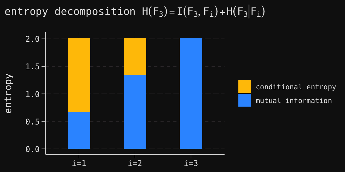
for each \(i=1,2,3\), and so the total entropy in \(\mathcal{F}_3\) decomposes into the sum of mutual information and conditional entropy. We visualize this decomposition for each of the three algebras in our filtration:
Code
# Create a data frame decomposing the entropy H(F3) into mutual information and conditional entropy# For each algebra F_i (i=1,2,3), we have: H(F3) = I(F3, F_i) + H(F3 | F_i)decomposition <-tibble(algebra =rep(c("i=1", "i=2", "i=3"), each =2), # Three algebras, each with two componentscomponent =rep(c("mutual information", "conditional entropy"), 3), # Two components per algebraentropy =c(H_F1, H_F3 - H_F1, H_F2, H_F3 - H_F2, H_F3, 0) # Values for each component)# Create a stacked bar chart showing the decomposition# Each bar represents H(F3) for a different conditioning algebra F_iggplot(decomposition, aes(x = algebra, y = entropy, fill = component)) +geom_col(width =0.4) +# Stacked column chartscale_fill_manual(name =NULL,values =c("mutual information"= blue, "conditional entropy"= yellow) ) +labs(title =TeX("entropy decomposition $H(F_3) = I(F_3, F_i) + H(F_3 | F_i)$"),x =NULL )
The decomposition \(H(\mathcal{F}_3) = I(\mathcal{F}_3, \mathcal{F}_i) + H(\mathcal{F}_3 \mid \mathcal{F}_i)\) reveals a fundamental trade-off: as we refine our information from \(\mathcal{F}_1\) to \(\mathcal{F}_2\) to \(\mathcal{F}_3\), mutual information increases (capturing more shared knowledge with the complete outcome) while conditional entropy decreases (leaving less residual uncertainty). The total entropy \(H(\mathcal{F}_3)\) remains constant, but its composition shifts as information accumulates.
Conclusion
We began this post by asking how to represent an observer’s information mathematically. The answer emerged through two complementary perspectives: algebras of sets, which capture the logical operations available to the observer, and partitions, which describe which outcomes can be distinguished from one another. Theorem 3 showed these views are equivalent—every algebra corresponds to a unique partition of atoms, and vice versa.
To quantify information, we introduced entropy as a measure of uncertainty associated with an algebra. The entropy \(H(\mathcal{G})\) tells us how much uncertainty remains when the observer’s knowledge is captured by \(\mathcal{G}\). Our coin-flip example illustrated how entropy increases as partitions refine: knowing the first flip yields \(H(\mathcal{F}_1) \approx 0.67\), knowing the first two flips yields \(H(\mathcal{F}_2) \approx 1.35\), and complete knowledge yields \(H(\mathcal{F}_3) \approx 2.02\).
We also introduced conditional entropy \(H(\mathcal{G} \mid \mathcal{H})\), measuring residual uncertainty in \(\mathcal{G}\) given knowledge of \(\mathcal{H}\), and mutual information \(I(\mathcal{G}, \mathcal{H})\), measuring information shared between algebras. These quantities satisfy the fundamental relationship
decomposing total uncertainty into shared information and residual uncertainty.
The framework of nested algebras representing evolving information has powerful applications beyond theoretical probability. In future posts, we’ll explore how these ideas illuminate gambling strategies and games of chance, where players accumulate information over time and make decisions under uncertainty. We’ll also see how the same mathematical structure underpins options pricing in mathematical finance, where nested filtrations model the information available to traders at different times, and conditional expectations with respect to these algebras determine fair prices for derivative securities. The interplay between information, uncertainty, and value in these contexts provides a rich testing ground for the concepts developed here.
Bibliography
Billingsley, P. 1995. Probability and Measure. Third. John Wiley & Sons, Inc.
Björk, T. 2020. Arbitrage Theory in Continuous Time. Fourth. Oxford Finance Series. Oxford University Press.
Walters, P. 1982. An Introduction to Ergodic Theory. Graduate Texts in Mathematics. Springer.