Brownian motion is the basic model of continuous random motion, first used to describe a particle buffeted by constant impacts from surrounding particles, and now the starting point for continuous-time pricing models in finance. This notebook builds it from the ground up. We begin with a discrete random walk, then shrink the time step \(\Delta t\to 0\) while scaling the step sizes so that the drift and variance stay finite. The Central Limit Theorem turns the net displacement into a normal random variable, which leads to the definitions of standard and arithmetic Brownian motion. SigAlg simulates both types, and each is illustrated with sampled trajectories.
Random walks
Consider a particle restricted to one-dimensional motion along an axis oriented in a vertical fashion, so that we speak of upward and downward movements. We suppose that the axis has been marked off, with a designated origin, so that we may specify its position at time \(t\) by giving a single coordinate \(X_t\). We fix a time interval \([a,b]\), divided into \(n\) subintervals of equal length \(\Delta t = (b-a)/n\). At teach time \[
t_k = a + k\Delta t, \quad k=0,1,\ldots,n-1,
\] we suppose that our particle experiences an impact from another particle, that will propel it either a distance of \(u+h\) units upward, or a distance of \(u-h\) units downward, for some \(u\) and \(h>0\). Thus, the displacements \[
\Delta X_{t_k} \stackrel{\text{def}}{=} X_{t_{k+1}} - X_{t_k}
\] are all equal to \(u+h\) or \(u-h\) (\(k=0,1,\ldots,n-1\)). We suppose that the upward and downward movements are equiprobable, and that the displacements are independent of each other. This leads us to consider the difference equations \[
\Delta X_{t_k} = u + h\, \Delta Z_{t_k}, \tag{1}
\] for \(k=0,1,\ldots,n-1\), where \(Z_t\) is a symmetric random walk with initial state \(0\). We call \(X_t\) a symmetric random walk with drift.
These types of random walks model a simplified version of Brownian motion in which a particle experiences a single impact per subinterval of time. For our time interval \([a,b]\) divided into \(n\) subintervals, the particle would experience \(n\) impacts. But in a true Brownian motion, these impacts are constant, and our ultimate goal is to model the net displacement \(X_b-X_a\) of the particle undergoing this type of motion over the time interval \([a,b]\). To do this, we let \(n\to\infty\) while holding the time interval fixed, which will force \(\Delta t\to 0\). However, if each impact propels the particle a fixed and unchanging distance \(u\pm h\), it is conceivable that the trajectory of the particle might be unbounded. So, to balance the number of particle impacts going to \(\infty\), we must correspondingly shrink \(u\) and \(h\).
The analysis goes like this. We sum both sides of the difference equation \((1)\) to get \[
X_b - X_a = \frac{u(b-a)}{\Delta t} + h \sum_{k=0}^{n-1} \Delta Z_{t_k}. \tag{2}
\] From this, we get formulas for the expectation and variance of the net displacement over the entire interval \([a,b]\): \[
E(X_b-X_a) = \frac{u(b-a)}{\Delta t}, \qquad V(X_b-X_a) = \frac{h^2(b-a)}{\Delta t}.
\] In order for the variance to not diverge to \(\infty\) as \(\Delta t \to 0\), we require that there is a positive real number \(\sigma^2\) (with units of squared length per time) such that \(h^2 = \sigma^2 \Delta t\); similarly, in order for the expectation to not diverge to \(\pm \infty\), we require that there is a real number \(\mu\) such that \(u = \mu \Delta t\) (with units of length per time). The number \(\mu\) is called a drift coefficient, while the positive square root \(\sigma = \sqrt{\sigma^2}\) is called a diffusion coefficient.
With chosen diffusion and drift coefficients, the difference equation (1) may be rewritten as \[
\Delta X_{t_k} = \mu\,\Delta t + \sigma \sqrt{\Delta t}\, \Delta Z_{t_k}.
\]
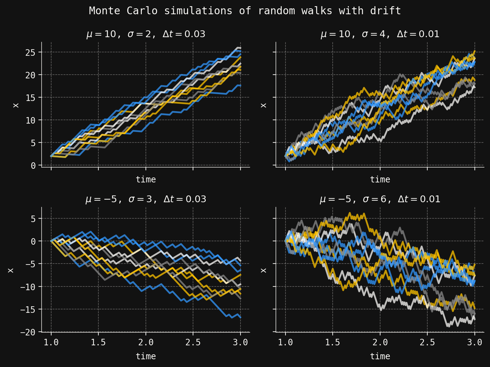
In the code cell below, we build several of these random walks by hand using SigAlg. Note the effects of the drift and diffusion coefficients.
We return to the net displacement \(X_b-X_a\) of our particle given in (2) with chosen drift and diffusion coefficients \(\mu\) and \(\sigma\): \[
X_b - X_a = \mu(b-a) + \sigma \left(\frac{\sum_{k=0}^{n-1} \sqrt{b-a}\, \Delta Z_{t_k}}{\sqrt{n}}\right).
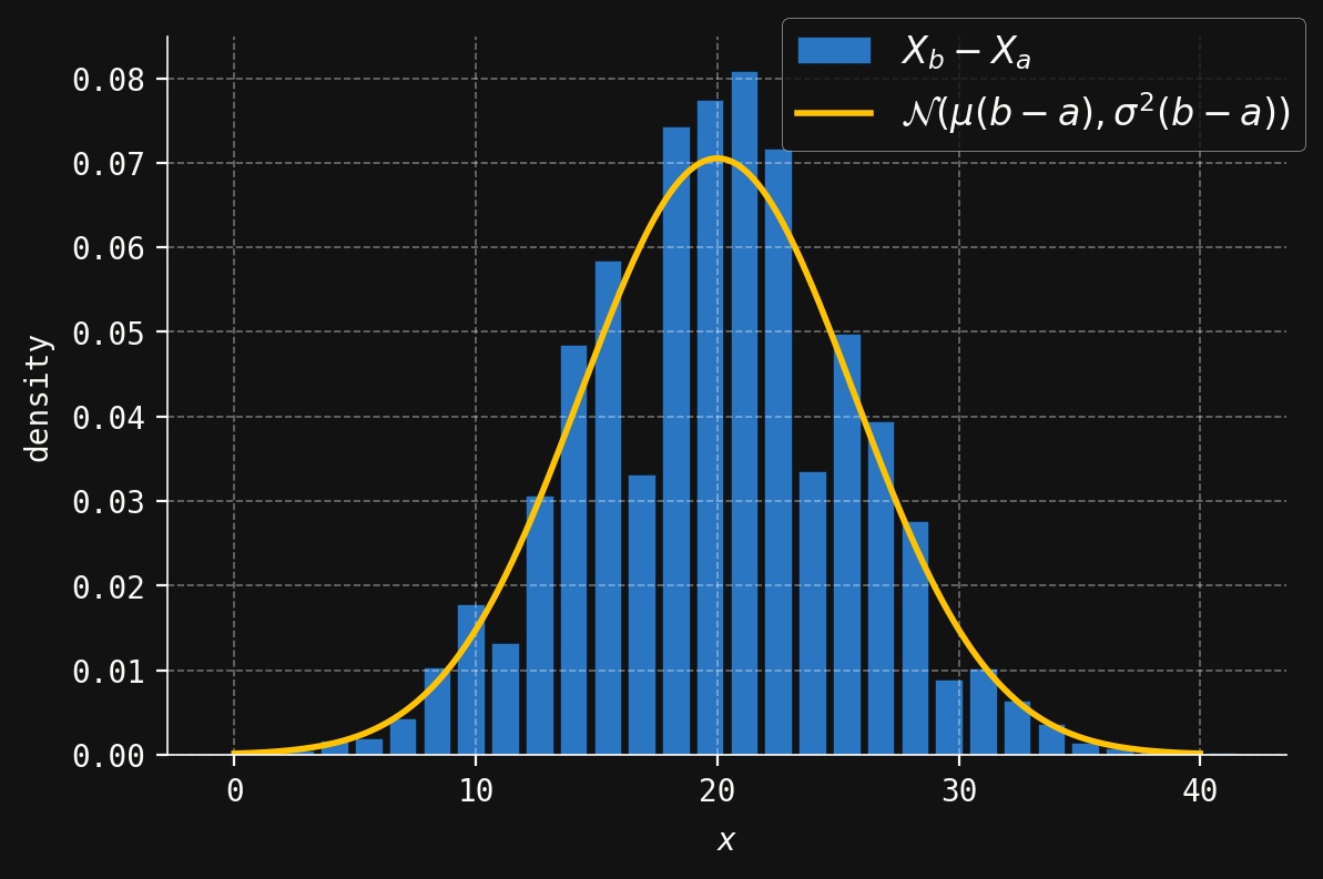
\] As we let the number \(n\) of particle impacts go to \(\infty\), the Central Limit Theorem applies to the random variable in parentheses, showing that it converges in distribution to an \(\mathcal{N}(0, b-a)\) random variable. Thus, in the limit, the net displacement \(X_b- X_a\) is an \(\mathcal{N}(\mu(b-a), \sigma^2(b-a))\) random variable.
For large \(n\) (i.e., small \(\Delta t\)) the net displacement is only approximately normal. We plot one such approximation in the next code cell.
Our disucssion has led us to the following. For a particle undergoing continuous impacts and experiencing true Brownian motion, it is natural to model its net displacement \(X_{t_2}-X_{t_1}\) over a time interval \([t_1,t_2]\) according to the equation \[
X_{t_2}-X_{t_1} = \mu(t_2-t_1) + \sigma(W_{t_2} - W_{t_1}),
\] where \(\mu\) and \(\sigma>0\) are parameters, and \(W_t\) is a continuous-time stochastic process, indexed by \(t\in [0,\infty)\), with the following properties:
The random variable \(W_0\) is deterministic, equal to \(0\).
For any \(0 \leq t_1 < t_2\), the random variable \(W_{t_2} - W_{t_1}\) is an \(\mathcal{N}(0, t-s)\) random variable.
For any \(0 \leq t_1 < t_2 < \cdots < t_n\), the random variables \(W_{t_2} - W_{t_1}, \ldots, W_{t_n} - W_{t_{n-1}}\) are independent.
The trajectories (i.e., sample paths) of the stochastic process are continuous.
A stochastic process \(W_t\) with these properties is called a standard Brownian motion, while the process \(X_t\) is called an arithmetic Brownian motion with drift parameter \(\mu\) and diffusion parameter \(\sigma\).
Whether or not such processes actually exist is a difficult matter. While they had appeared before in papers of Thiele (1880), Bachelier (1900) and Einstein (1905), it was Wiener (1923) who first provided a rigorous construction leading to them also being called Wiener processes. To see part of the difficulty in proving the existence of a Brownian motion, note that the standard deviation of the random variable \(W_{t_2} - W_{t_1}\) is \(\sqrt{t_2 - t_1}\). If we use this quantity as a proxy for the net displacement of a particle, then dividing it by \(t_2-t_1\) would serve as a measure of the average velocity of the particle over the time interval \([t_1,t_2]\). But this velocity blows up to \(\infty\) as \(t_2\to t_1\), suggesting that a particle undergoing Brownian motion has extremely erratic behavior. This also suggests that the techniques of classical calculus will be inadequate to treat Brownian motion, and that a new stochastic calculus will be required.
SigAlg provides a method BrownianMotion for simulating standard and arithmetic Brownian motions. To describe it, suppose we partition a time interval \([a,b]\) as \[
a = t_0 < t_1 < \cdots < t_n = b,
\] in such a way that the lengths \(\Delta t = t_{k+1}-t_k\) are constant for each \(k=0,1,\ldots,n-1\). Taking \(W_a=0\), we then have \[
W_{t_k} = \sum_{j=0}^{k-1} (W_{t_{j+1}} - W_{t_j}).
\] Given the partition of \([a,b]\) above, SigAlg samples from the random variables \(W_{t_{j+1}} - W_{t_j} \sim \mathcal{N}(0,\Delta t)\) and sums them to produce a sample from \(W_{t_k}\). These samples are then combined into a discrete approximation of the standard Brownian motion. A similar technique is used to simulate arithmetic Brownian motions.
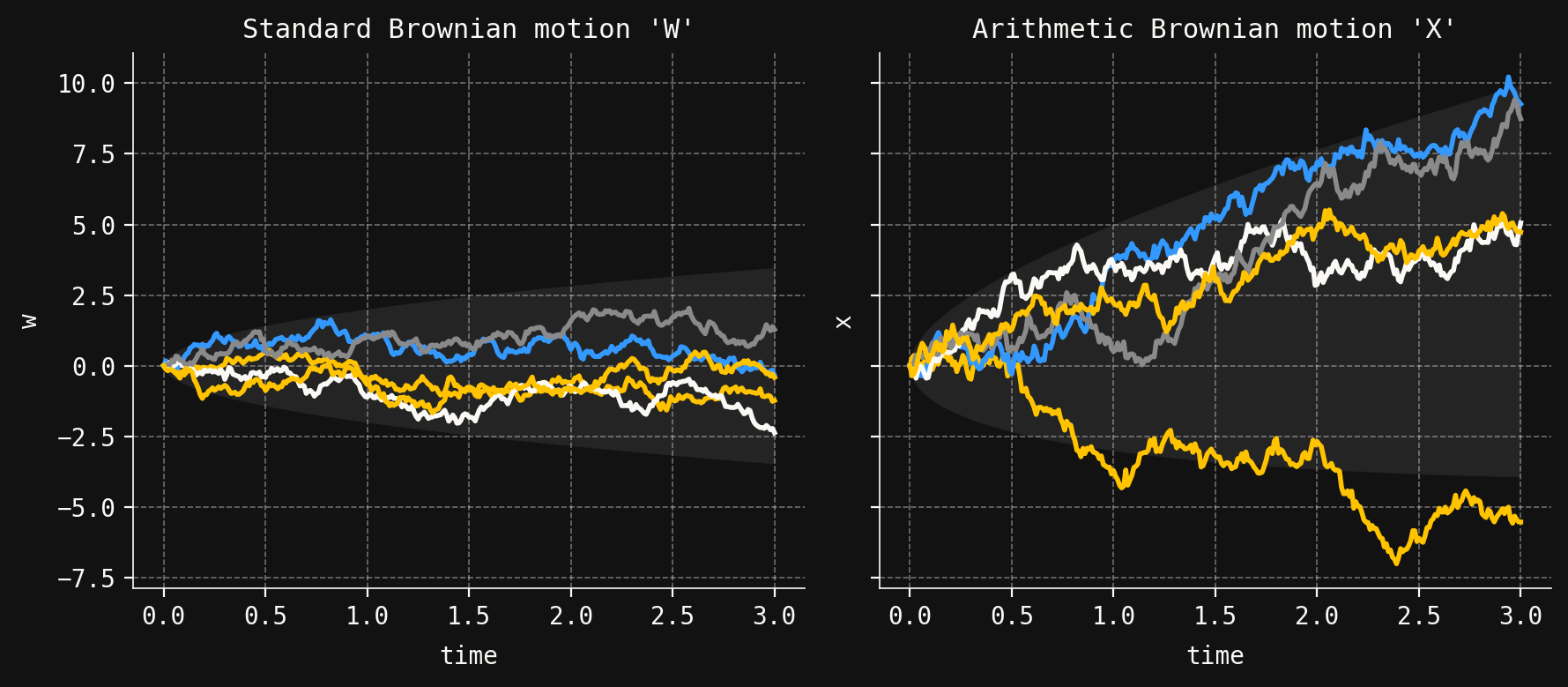
In the next code cell, we plot sampled trajectories of standard and arithmetic Brownian motions, over the time interval \([0,3]\) with \(\Delta t=0.01\), and with drift and diffusion coefficients \(\mu=1\) and \(\sigma=2\). To show the statistical trends of the trajectories, the gray bands plot the regions bounded by \(\pm 2 \sqrt{t}\) for the standard motion, and \(\mu t \pm 2\sigma \sqrt{t}\) for the arithmetic one. For a given \(t\), these are the regions within two standard deviations of the mean.